1 Theoretical overview: how TRIGRS “thinks”

Before installing and running anything, it pays to understand what TRIGRS computes and why. This chapter is a simplified, teaching-oriented version of the theory — readers who want the full rigor should read the program manual (Baum, Savage & Godt, 2008 — USGS OFR 2008-1159) and the reference paper by Baum, Godt & Savage (2010), both listed in the References.

1.1 The physical problem in one sentence

Rain infiltrates → water fills the soil pores → pore-water pressure rises → friction between the grains decreases → at some point the slope fails.

Shallow rainfall-induced landslides (typically 1 to 3 m deep) are the dominant mechanism in disasters such as the one that struck the Rio de Janeiro Highlands in January 2011. The failure surface usually forms at the contact between the soil (colluvium/residual soil) and a less permeable material below — and this is exactly the setting that TRIGRS represents.

For each cell of a raster grid and for each instant of a rainstorm, TRIGRS answers the question “is this cell stable right now?” by combining two ingredients:

a transient infiltration model (how pore-water pressure evolves in time and with depth), and
an infinite-slope stability model (does the computed pressure lower the factor of safety?).

Let us look at each of them.

1.2 Ingredient 1 — the infinite slope

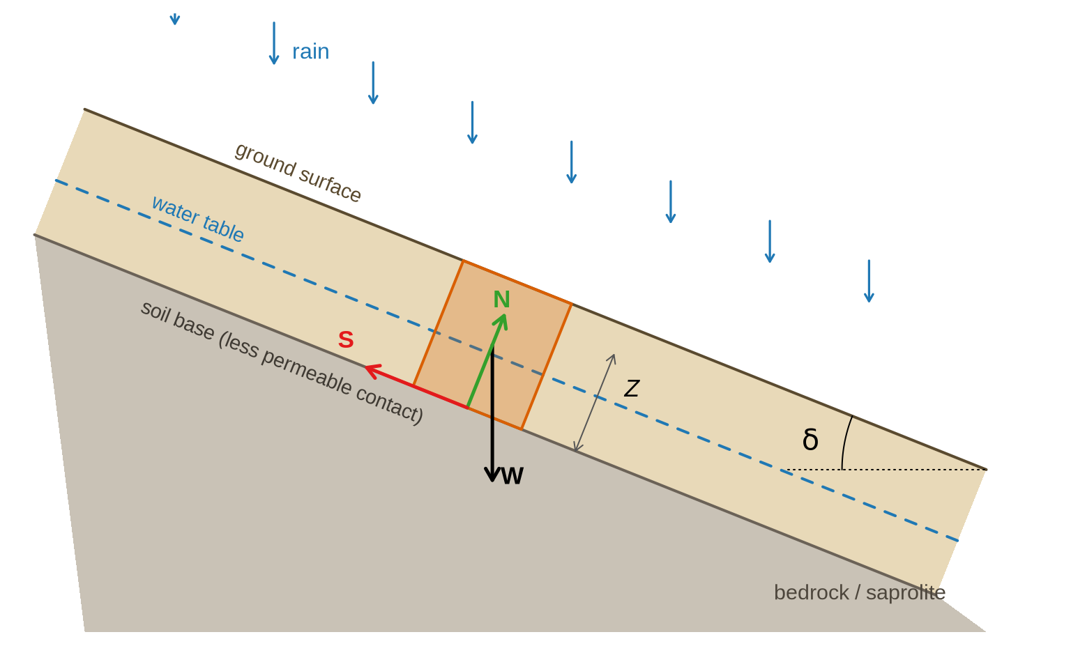
The geometry of shallow landslides (length much greater than thickness) allows a powerful simplification: treating each cell as an infinite inclined plane, with failure parallel to the ground surface. Figure 1.1 shows the setup:

Figure 1.1: Sketch of the infinite-slope model used by TRIGRS. The soil column of depth Z, inclined at an angle δ, is loaded by its weight (W) and resists through friction and cohesion at its base. The water table (dashed blue line) controls the pressure head ψ on the potential failure surface.

The equilibrium of this column leads to the Factor of Safety formula that TRIGRS evaluates at each depth \(Z\) and time \(t\) (Baum et al., 2010, eq. 4):

\[ FS(Z,t) \;=\; \underbrace{\frac{\tan\varphi'}{\tan\delta}}_{\text{friction}} \;+\; \underbrace{\frac{c'}{\gamma_s\, Z \sin\delta \cos\delta}}_{\text{cohesion}} \;-\; \underbrace{\frac{\psi(Z,t)\,\gamma_w \tan\varphi'}{\gamma_s\, Z \sin\delta \cos\delta}}_{\text{effect of water}} \]

Term	Meaning	Where it comes from
\(\delta\)	slope angle	slope grid (`slope.asc`)
\(\varphi'\)	effective friction angle of the soil	laboratory tests/literature (per zone)
\(c'\)	effective cohesion	laboratory tests/literature (per zone)
\(\gamma_s\), \(\gamma_w\)	unit weight of soil and of water	tests/constant
\(Z\)	depth being evaluated	down to `zmax.asc`
\(\psi(Z,t)\)	pressure head	this is what the infiltration model computes!

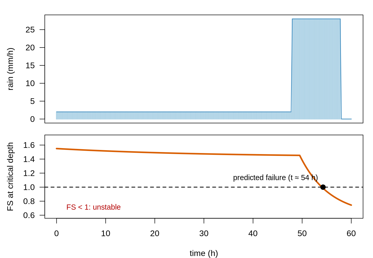
Read the equation as a contest: friction + cohesion (stabilizing) against the effect of water (destabilizing). The first two terms are constant in time; the third grows during the rainstorm because \(\psi\) grows. When \(FS\) drops below 1, the cell is predicted to be unstable. Note also the role of \(Z\): the deeper the surface, the smaller the relative weight of cohesion — which is why there is a “critical” depth at which \(FS\) is minimum (TRIGRS reports it in the TRz_at_fs_min grid).

1.3 Ingredient 2 — transient infiltration

The central piece is still missing: how does \(\psi(Z,t)\) evolve during the rainstorm? TRIGRS uses analytical solutions of the equation for vertical flow in a porous medium (the linearized Richards equation, following Iverson, 2000, as extended by Baum et al., 2008; 2010): the infiltrating rain generates a “pressure wave” that diffuses downward at a rate controlled by the soil’s hydraulic diffusivity \(D_0\).

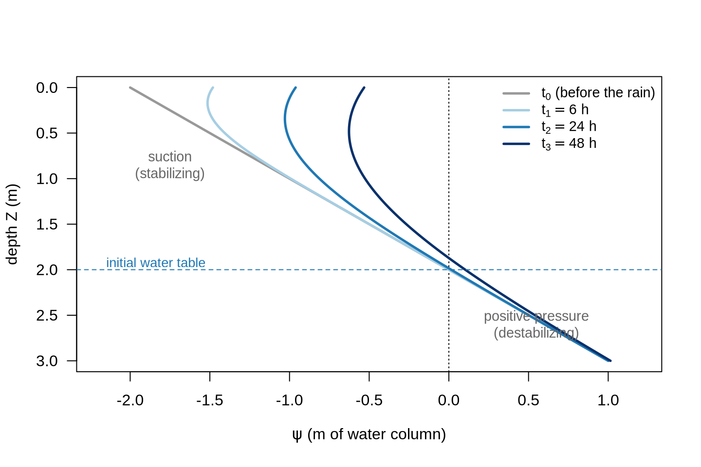
Figure 1.2: Concept of the transient response: pressure-head profiles ψ(Z) at successive times during a rainstorm. The initial condition (t₀) has negative pressure (suction) above the water table; as rain infiltrates, the ‘pressure front’ advances downward (t₁, t₂, t₃) and reduces suction — and may generate positive pressure. Conceptual curves based on the linearized diffusion solution.

Points worth remembering (all detailed in the manual and in Baum et al., 2010):

Unsaturated zone: above the water table the soil is under suction (negative pressure), which helps stability. TRIGRS can model this zone explicitly (Gardner model, parameter \(\alpha\)) or assume the soil is saturated from the start (more conservative).
Diffusivity \(D_0\) controls the delay of the response: more permeable soils respond within hours; less permeable ones, within days. This is why TRIGRS can predict the timing of instability, not just its location.
Lower boundary: the impermeable base at zmax makes the pressure “build up” — a finite-depth model, one of the TRIGRS extensions to Iverson’s original model.
Infiltration limit: if rainfall exceeds the infiltration capacity (\(K_{sat}\)), the excess becomes surface runoff, routed from cell to cell with the D8 scheme computed by TopoIndex.

Combining the two ingredients yields the typical signature of a cell’s response:

Figure 1.3: Conceptual response of a cell during an event: the hyetograph (top) drives infiltration; pore pressure at the critical depth rises with a lag and FS drops. The cell ‘fails’ when FS < 1 — TRIGRS provides both the timing and the location.

1.4 From critical depth to mobilizable volume (the role of Vdy2)

At a given instant of the rainstorm, each cell has a complete \(FS(Z)\) profile — from the top of the soil down to zmax. The depth at which \(FS\) is minimum is the critical depth \(Z_{cr}\): that is where failure tends to occur, typically where the pressure front meets the lowest relative resistance. TRIGRS delivers both pieces of information in separate grids:

TRfs_min → the minimum FS of the cell (unstable if < 1);
TRz_at_fs_min → the critical depth \(Z_{cr}\) of that cell (in meters).

Figure 1.4 illustrates the concept for four neighboring cells at the same instant of a rainstorm:

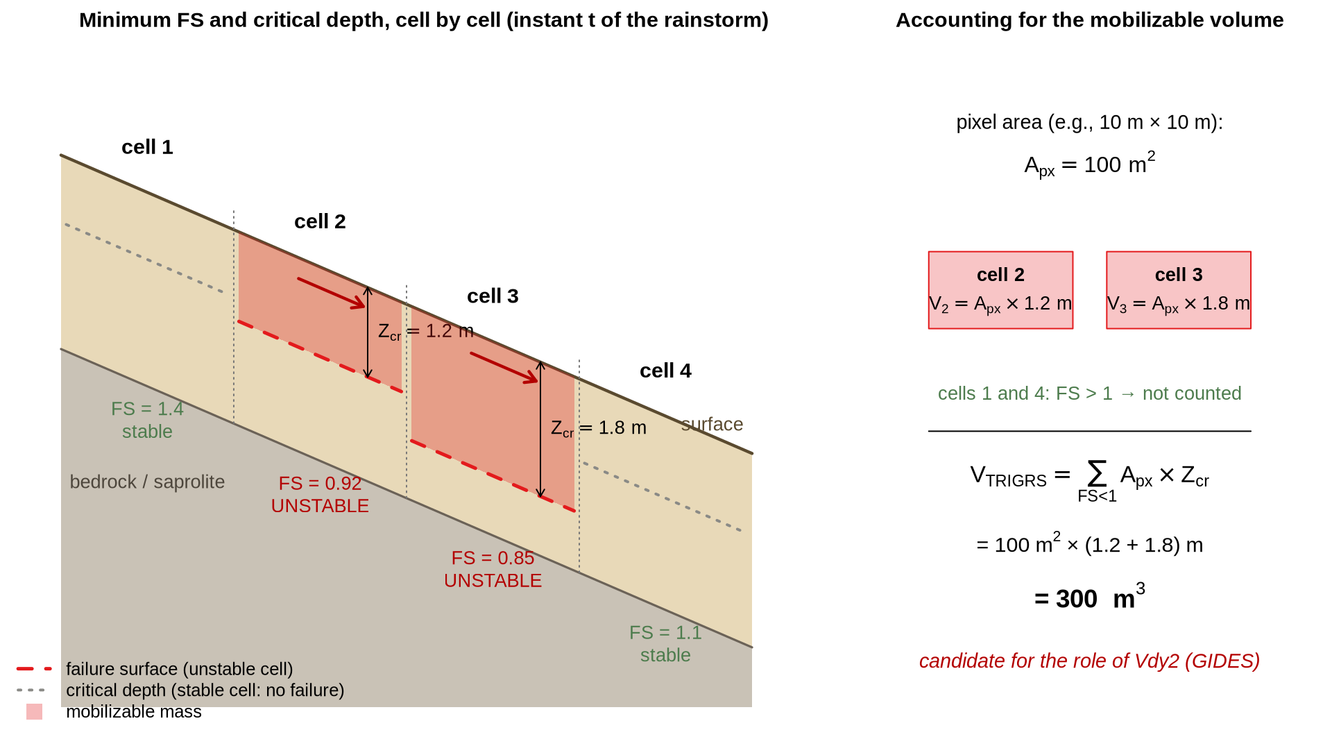
Figure 1.4: Failure model for a given rainfall, at a given instant, in four neighboring cells. Each cell has its own minimum FS and critical depth Z_cr (TRz_at_fs_min grid). In the unstable cells (FS < 1, in red), the prism above the failure surface is the mobilizable material: volume = pixel area × Z_cr. Summing the prisms of all unstable cells gives the mobilizable volume estimated by TRIGRS — a candidate for the role of Vdy2 in the GIDES methodology.

Reading the figure gives the complete recipe of the proposed methodology:

Run TRIGRS with the rainfall of interest (the observed event, or the design rainfall for a given return period — the same \(P_d\) that GIDES uses in Vdy2);
At the instant analyzed, select the cells with FS < 1 (TRfs_min grid);
Extract the critical depth \(Z_{cr}\) of those cells (TRz_at_fs_min grid);
The mobilizable volume of each pixel is the pixel area times its critical depth — and the total is the sum:

\[ V_{TRIGRS}(t) \;=\; \sum_{i \,:\, FS_i(t) < 1} A_{px} \cdot Z_{cr,i}(t) \]

where \(A_{px}\) is the cell area (resolution², e.g., a 10 m grid → 100 m² per pixel).

1.4.1 How the GIDES manual accounts for volumes

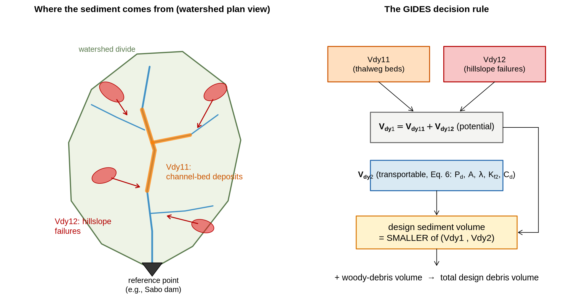
To understand where this \(V_{TRIGRS}\) fits, we need to see how the Technical Manual for the Design of Debris-Flow Interventions (Manual Técnico para Concepção de Intervenções para Fluxo de Detritos; JICA/MI, 2018 — GIDES Project) estimates the sediment volume that reaches the watershed’s reference point (for example, where a Sabo dam is planned). The manual compares two volumes and adopts the smaller one:

① Vdy1 — what the watershed CAN produce (potential volume), with two components surveyed in the field (Section 2.5.1.1 of the manual):

Vdy11 — channel-bed sediment: material already deposited along the thalwegs that can be entrained (estimated from channel cross sections: width × mobilizable thickness × length);
Vdy12 — sediment from hillslope failures: hillslope areas that may fail during the event × soil thickness — currently estimated through field inspection and inventories.

② Vdy2 — what the rainfall CAN transport (transportable volume, Section 2.5.1.2, Equation 6 — an empirical correlation based on Japanese experience):

\[ V_{dy2} \;=\; \frac{10^3 \cdot P_d \cdot A}{1-\lambda} \;\cdot\; K_{f2} \;\cdot\; \frac{C_d}{1-C_d} \]

Term	Meaning	How it is obtained
\(P_d\)	maximum daily precipitation (mm) for the adopted return period (at least 100 years for Sabo works)	rainfall frequency analysis
\(A\)	watershed area (km²)	GIS
\(\lambda\)	deposit porosity (≈ 0.4)	manual default
\(K_{f2}\)	runoff correction factor (0.1–0.5)	chart × watershed area (Fig. 14 of the manual)
\(C_d\)	debris-flow concentration	equilibrium formula in the manual’s annex

Figure 1.5 summarizes the accounting (redrawn from the manual’s concept):

Figure 1.5: Volume accounting in the GIDES methodology (adapted from JICA/MI, 2018). Left: the watershed in plan view — sediment comes from the thalweg beds (Vdy11, orange) and from hillslope failures (Vdy12, red), and is measured at the reference point. Right: the design volume is the SMALLER of the potential volume (Vdy1) and the volume transportable by the design rainfall (Vdy2), plus the woody-debris volume.

1.4.2 Where TRIGRS fits into this accounting

Note the weak link of the empirical path: Vdy12 depends on field inspection and inventories (what failed in the past), and Vdy2 is a correlation fitted to events in Japan. The research proposal is to use TRIGRS as a parallel physically based path, driven by the same design rainfall \(P_d\):

flowchart TB
  PD["Design rainfall P_d (adopted return period)"]

  subgraph EMP["Empirical path (GIDES)"]
    CAMPO["Field survey /<br/>inventory"] --> V11["Vdy11<br/>(channel bed)"]
    CAMPO --> V12["Vdy12<br/>(hillslope failures)"]
    V11 --> V1["Vdy1 = Vdy11 + Vdy12"]
    V12 --> V1
    EQ6["Equation 6<br/>(empirical, Japan)"] --> V2["Vdy2<br/>(transportable)"]
    V1 --> MIN["design volume =<br/>min(Vdy1, Vdy2)"]
    V2 --> MIN
  end

  subgraph FIS["Physical path (TRIGRS)"]
    TRG["TRIGRS: FS(Z,t)<br/>with the P_d hyetograph"] --> ZC["cells with FS &lt; 1 +<br/>critical depth Z_cr"]
    ZC --> VT["V_TRIGRS = Σ A_px·Z_cr<br/>× 1/(1−λ)"]
  end

  PD --> EQ6
  PD --> TRG
  VT -. "physically based estimate of Vdy12" .-> V12
  VT -. "confrontation / validation" .-> V2
  MIN --> OBRA["design of the interventions"]

  classDef default fill:#ffffff,stroke:#64748b,color:#111827
  style EMP fill:#f8fafc,stroke:#94a3b8,color:#0f172a
  style FIS fill:#dbeafe,stroke:#1f78b4,color:#0f172a
  style PD fill:#fff3cd,stroke:#d97706,color:#0f172a

Connection between the GIDES methodology (empirical path, on the left) and the TRIGRS-based proposal (physical path, on the right). Both start from the same design rainfall Pd; V_TRIGRS can replace/refine Vdy12, be confronted with Vdy2, and propagate climate-change scenarios.

On three fronts:

Replace/refine Vdy12: instead of relying only on the inventory of past events, TRIGRS tells which slopes fail under the design rainfall and how thick the failed mass is — a physically based estimate, specific to the watershed and to the rainfall;
Confront Vdy2: Equation 6 was calibrated in Japan; comparing \(V_{TRIGRS}\) with Vdy2 in the watersheds of the Rio de Janeiro Highlands tests whether the correlation transfers to the Brazilian context (and the 2011 event provides the ground truth);
Climate change: since rainfall enters both paths explicitly (through \(P_d\)), it suffices to scale up the design rainfall by the climate-change factors and propagate it — the volumes respond physically, not by extrapolating the correlation.

Two caveats when comparing with Vdy2

Bulking/porosity: \(V_{TRIGRS}\) is an in situ soil volume; the Vdy2 of the GIDES manual refers to transported sediment including voids (the factor \(1/(1-\lambda)\), with \(\lambda \approx 0.4\)). To compare them on the same basis, the same correction is applied.
Mobilized ≠ transported: TRIGRS estimates what fails on the hillslopes; how much of that material actually reaches the reference point is the propagation step — in the comparison with Vdy1/Vdy2 (GIDES adopts the smaller of the two), this difference is part of the research discussion.

This is exactly the calculation we will carry out, in practice, in the chapter First run and results — which ends by mapping the mobilizable volume cell by cell and applying the comparison with V_dy2 to the tutorial example.

1.5 Assumptions and limitations (read before trusting the map!)

The TRIGRS manual is emphatic: the program is a tool for those who understand the phenomenon, and interpreting its results requires geological and geotechnical judgment. The main simplifications are:

1-D vertical flow and isotropic/homogeneous soil within each cell (heterogeneity only between cells/zones);
infinite-slope model: valid for shallow, planar failures — not for deep-seated or rotational landslides;
no propagation (runout) modeling of the mobilized mass — TRIGRS tells where failures initiate and how much material becomes unstable; what happens downslope is the subject of the debris-flow methodology (Parts 3 and 4 of this short course);
results are only as good as the input data (DEM, soil depth, geotechnical parameters, rainfall) — hence the importance of calibrating against a landslide-scar inventory.

1.6 The overall methodology flowchart

The diagram below organizes all the steps of the work — from data collection to the estimation of volumes under climate change. It expands the initial research outline and serves as a map for the entire short course:

flowchart TB
  subgraph ETAPA1["1 · Data collection (GIS)"]
    direction TB
    A1["DEM<br/>(slope, flow direction)"]
    A2["Geological, geomorphological<br/>and soil maps"]
    A3["Land use<br/>and land cover"]
    A4["Rainfall<br/>(event and IDF)"]
    A5["Landslide-scar<br/>inventory (2011)"]
  end

  subgraph ETAPA2["2 · Geospatial analysis"]
    B1["Property zones<br/>(zones.asc)"]
    B2["Soil depth<br/>(zmax.asc)"]
    B3["Congruent grids<br/>(GridMatch)"]
  end

  subgraph ETAPA3["3 · TRIGRS modeling"]
    C1["TopoIndex<br/>(D8 routing)"]
    C2["TRIGRS<br/>FS(Z,t) per cell"]
  end

  subgraph ETAPA4["4 · Validation and calibration"]
    D1["Comparison of FS < 1<br/>× scars"]
    D2["Parameter adjustment<br/>(K_sat, initial water table, c', φ')"]
  end

  subgraph ETAPA5["5 · Products"]
    E1["Calibrated susceptibility<br/>map"]
    E2["Mobilizable volume<br/>Σ area × Z_failure"]
    E3["GIDES/JICA volumes<br/>(Vdy1, Vdy2)"]
    E4["Climate-change<br/>scenarios (rainfall Pd)"]
  end

  ETAPA1 --> ETAPA2 --> C1 --> C2 --> D1 --> D2
  D2 -- "iterate" --> C2
  D2 --> E1
  E1 --> E2 --> E3
  A4 --> E4 --> C2
  E4 --> E3

  classDef default fill:#ffffff,stroke:#64748b,color:#111827
  style ETAPA1 fill:#f8fafc,stroke:#94a3b8,color:#0f172a
  style ETAPA2 fill:#f8fafc,stroke:#94a3b8,color:#0f172a
  style ETAPA3 fill:#dbeafe,stroke:#1f78b4,color:#0f172a
  style ETAPA4 fill:#f8fafc,stroke:#94a3b8,color:#0f172a
  style ETAPA5 fill:#fef3c7,stroke:#d97706,color:#0f172a

Overall flowchart of the research methodology. In blue, the steps covered by Part 1 of the short course; the other parts follow the numbering shown.

And, within the modeling step, the operational workflow of the programs you will use in the next chapters:

flowchart LR
  G["GIS<br/>(QGIS/ArcGIS)<br/>.asc grids"] --> M["GridMatch<br/><i>congruent grids?</i>"]
  M --> T["TopoIndex<br/>tpx_in.txt<br/><i>D8 indices + weights</i>"]
  T --> R["TRIGRS<br/>tr_in.txt<br/><i>infiltration + FS</i>"]
  R --> S["Results<br/>TRfs_min, TRz_at_fs_min,<br/>TRp_at_fs_min, runoff..."]
  S --> V["Visualization and analysis<br/>(R/terra or QGIS)"]

  classDef default fill:#ffffff,stroke:#64748b,color:#111827
  style R fill:#dbeafe,stroke:#1f78b4,color:#0f172a

Operational workflow: from GIS rasters to result maps. This is exactly the sequence we will run in the tutorial example.

1.7 Where each topic is covered in the short course

Flowchart step	Where it is covered
Installing and compiling the tools	Installation and Compilation
Understanding the grids and input files	The tutorial example
Running TopoIndex + TRIGRS, visualizing FS, and quantifying volumes	First run and results
Real watershed, calibration, volumes, climate	Parts 2–4 (under construction)