5 First run and results

In this chapter we run TRIGRS on the tutorial example and analyze everything it produces — from the factor-of-safety map to the mobilizable volume cell by cell, closing with the application of the research proposal (the role of V_dy2).

5.1 Preparation

Clone (or download) this repository.
Copy the topoindex.exe and trigrs.exe executables compiled in the Compilation chapter into the exemplo_01\ folder.
Make sure the exemplo_01\Resultados\ folder exists.

5.2 Run

Open PowerShell in the exemplo_01\ folder and run the two programs, in this order:

.\topoindex.exe    # reads tpx_in.txt -> writes data\TI*_tutorial.* (D8 indices and weights)
.\trigrs.exe       # reads tr_in.txt  -> writes Resultados\TR*.asc

Each run takes ~1 second on this toy grid. TopoIndex defines the computation order of surface runoff (D8), the runoff distribution weights, and the array sizes; TRIGRS performs the transient infiltration and stability analysis. The expected outputs end with:

 No grid mismatch found!    <- TopoIndex: congruent grids
 ...
 TRIGRS finished!           <- TRIGRS: run completed

5.3 What was produced

In exemplo_01\Resultados\:

File	Contents
`TRfs_min_tutorial_1.asc`, `_2.asc`	Minimum FS per cell at the output times (48 h and 60 h)
`TRz_at_fs_min_*.asc`	Critical depth Z_cr (m) — where the minimum FS occurs
`TRp_at_fs_min_*.asc`	Pore pressure (m of water column) at the critical depth
`TRwater_depth_*.asc`	Simulated water-table depth
`TRrunoffPer.asc`, `TRinfilratPer.asc`	Runoff and infiltration rate per rainfall period
`TRlist_z_p_fs_tutorial.txt`	Detailed Z–P–FS listing per cell (vertical profiles)
`TrigrsLog.txt`	Run log — always check warnings and the mass balance (written to `exemplo_01\` itself, not to `Resultados\`)

The .asc rasters open directly in QGIS (drag and drop) — or in R, as we will do now.

5.4 Factor of safety during the rainstorm

library(terra)

fs48 <- rast("../exemplo_01/Resultados/TRfs_min_tutorial_1.asc")  # t = 48 h
fs60 <- rast("../exemplo_01/Resultados/TRfs_min_tutorial_2.asc")  # t = 60 h

# TRIGRS caps FS at 10 (stable cells); we bin the color scale for readability
brks <- c(0, 0.8, 1.0, 1.2, 1.5, 2, 3, 10)
cols <- hcl.colors(length(brks) - 1, "RdYlGn")

par(mfrow = c(1, 2))
plot(fs48, main = "Minimum FS — 48 h", breaks = brks, col = cols)
plot(fs60, main = "Min. FS — 60 h (end of rain)", breaks = brks, col = cols)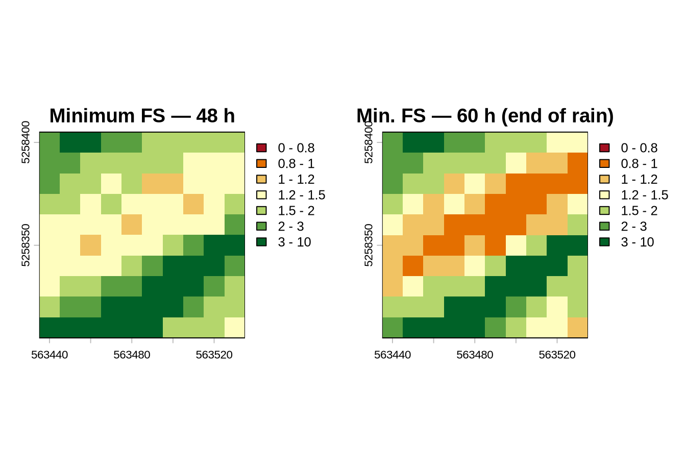

Minimum FS per cell at the two output times. Cells with FS < 1 (red–orange classes) are predicted to be unstable.

Compare the two times: during the first 48 h (light rain) practically everything is stable; in the final 12 h, with the storm, infiltration raises the pore pressure and FS plunges in the steepest cells.

5.5 Where, and at what depth, would it fail?

The TRz_at_fs_min grid is the critical depth Z_cr of each cell — the concept of Figure 1.4 in the theory chapter coming out of the model:

zfs <- rast("../exemplo_01/Resultados/TRz_at_fs_min_tutorial_2.asc")
pfs <- rast("../exemplo_01/Resultados/TRp_at_fs_min_tutorial_2.asc")

par(mfrow = c(1, 2))
plot(zfs, main = "Critical depth Z_cr (m)",
     col = hcl.colors(25, "Blues", rev = TRUE))
plot(pfs, main = "Pore pressure at Z_cr (m)",
     col = hcl.colors(25, "PuBuGn", rev = TRUE))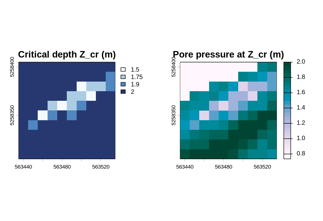

Left: critical depth Z_cr (where FS is minimum) — the thickness of the mass that tends to fail. Right: pore pressure acting at that depth.

5.6 The mobilizable volume of each cell

Now the central step of the proposal: in the unstable cells (FS < 1), the product pixel area × Z_cr is the volume that the cell can mobilize. We build the cell-by-cell volume map:

area_celula <- prod(res(fs60))                    # m² per cell (here: 10 m x 10 m = 100 m²)

zcr_inst <- ifel(fs60 < 1, zfs, NA)               # Z_cr of the unstable cells only
vol_px   <- zcr_inst * area_celula                # m³ per cell

par(mfrow = c(1, 2))
plot(zcr_inst, main = "Z_cr, unstable cells (m)",
     col = hcl.colors(25, "Blues", rev = TRUE))
plot(vol_px, main = "Volume per cell (m³)",
     col = hcl.colors(25, "Reds", rev = TRUE))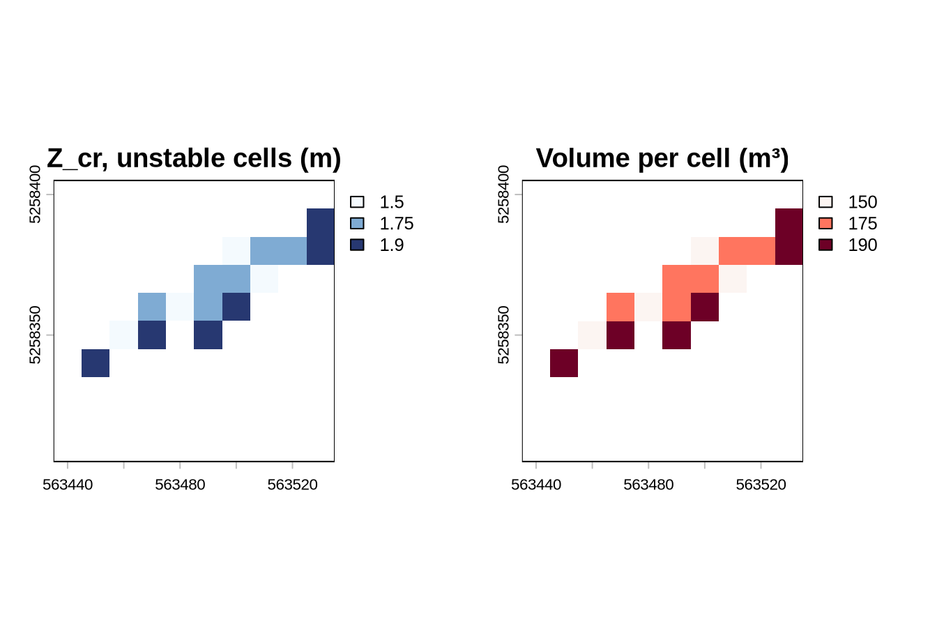

Left: critical depth of the unstable cells only (FS < 1). Right: mobilizable volume of each cell (pixel area × Z_cr) — the sum of this map is V_TRIGRS.

n_inst  <- global(fs60 < 1, "sum", na.rm = TRUE)[1, 1]
z_medio <- global(zcr_inst, "mean", na.rm = TRUE)[1, 1]

data.frame(
  unstable_cells        = n_inst,
  unstable_area_m2      = n_inst * area_celula,
  mean_failure_depth_m  = round(z_medio, 2),
  mobilizable_volume_m3 = round(global(vol_px, "sum", na.rm = TRUE)[1, 1], 1)
)

  unstable_cells unstable_area_m2 mean_failure_depth_m mobilizable_volume_m3
1             16             1600                 1.74                  2790

5.7 Applying the proposal: from TRIGRS to Vdy2

We close the loop by reproducing, on the tutorial grid, the two paths described in the theory: the physical path (V_TRIGRS) and the empirical path of the GIDES manual (V_dy2, Equation 6), and comparing them at the end as a designer would.

Illustrative numbers!

The tutorial grid is synthetic (100 cells of 10 m) and the example rainfall is unrealistic on purpose (the storm amounts to hundreds of mm/h, for the USGS’s teaching purposes). We therefore adopt here an illustrative design rainfall of \(P_d\) = 180 mm/day and typical values of \(K_{f2}\) and \(C_d\). What matters is the procedure — in the real watersheds of the research, each of these numbers will be obtained from the local frequency analysis and from the manual.

5.7.1 Step 1 — Physical mobilizable volume (V_TRIGRS)

lambda <- 0.4                                    # deposit porosity (GIDES manual)

V_insitu <- global(vol_px, "sum", na.rm = TRUE)[1, 1]  # intact soil that fails (m3)
V_solto  <- V_insitu / (1 - lambda)              # corrected to volume with voids (bulked)

cat("Unstable cells (FS<1):", n_inst,
    "\nV in situ =", round(V_insitu), "m³",
    "\nV bulked  =", round(V_solto), "m³  (comparable to the GIDES volumes)\n")

Unstable cells (FS<1): 16 
V in situ = 2790 m³ 
V bulked  = 4650 m³  (comparable to the GIDES volumes)

The \(1/(1-\lambda)\) correction puts the volume on the same basis as the manual: GIDES works with deposited sediment, including voids, not with the intact soil of the hillslope.

5.7.2 Step 2 — Empirical transportable volume (V_dy2, Equation 6)

# watershed area = valid cells x cell area (in km2)
n_total <- global(!is.na(fs60), "sum")[1, 1]
A_km2   <- n_total * area_celula / 1e6

Pd  <- 180    # mm/day -- ILLUSTRATIVE design rainfall (return period set by the frequency analysis)
Kf2 <- 0.5    # correction factor: upper bound, typical of very small watersheds (Fig. 14)
Cd  <- 0.35   # debris-flow concentration (equilibrium formula in the manual's annex)

Vdy2 <- 1e3 * Pd * A_km2 / (1 - lambda) * Kf2 * Cd / (1 - Cd)

cat("Watershed area A =", A_km2, "km²",
    "\nVdy2 = 10³ ×", Pd, "×", A_km2, "/ (1 −", lambda, ") ×", Kf2,
    "×", Cd, "/ (1 −", Cd, ") =", round(Vdy2), "m³\n")

Watershed area A = 0.01 km² 
Vdy2 = 10³ × 180 × 0.01 / (1 − 0.4 ) × 0.5 × 0.35 / (1 − 0.35 ) = 808 m³

5.7.3 Step 3 — The confrontation (the smaller-value rule)

data.frame(
  path      = c("physical (TRIGRS, bulked)", "empirical (Vdy2, Eq. 6)"),
  volume_m3 = round(c(V_solto, Vdy2)),
  role      = c("what the slopes mobilize for this rain",
                "what the rain can transport")
)

                       path volume_m3                                   role
1 physical (TRIGRS, bulked)      4650 what the slopes mobilize for this rain
2   empirical (Vdy2, Eq. 6)       808            what the rain can transport

cat("\nVolume to adopt (smaller-value rule, analogous to GIDES):",
    round(min(V_solto, Vdy2)), "m³\n")


Volume to adopt (smaller-value rule, analogous to GIDES): 808 m³

Reading the result: if \(V_{TRIGRS} > V_{dy2}\), the hillslopes produce more sediment than the rainfall can transport — transport is the limiting factor (a transport-limited scenario); if \(V_{TRIGRS} < V_{dy2}\), sediment production on the hillslopes is the bottleneck (supply-limited). This comparison — physics on one side, a Japanese correlation on the other — is exactly the experiment the research will carry out in the real watersheds, with the advantage that, by changing only \(P_d\) (for instance, scaled up by climate scenarios), both paths respond consistently.