8  Case study 3 — Petrópolis (Alto da Serra/Morin)

This chapter applies the methodology of the short course to the third case in the Rio de Janeiro Highlands (Região Serrana): the forested valley that descends from the Serra dos Órgãos range to the Morin neighborhood, in Alto da Serra (1st District of Petrópolis), scene of the disaster of February 15, 2022. The sequence is the same as in the Nova Friburgo and Teresópolis chapters: context, Sabo dam site, input data, watershed, design rainfall, climate change, and the traditional GIDES/JICA method (sections 8.1 to 8.7); then the TRIGRS modeling, the calibration against the 2022 landslide scars, the V_TRIGRS → V_dy12 coupling, the synthesis, and the reproducibility notes (sections 8.8 to 8.12).

NoteHow to read this chapter

Every number in the text comes from a file of the project pipeline (folder data/cases/petropolis/ of the companion) or from a cited reference. In sections 8.1 to 8.7, the values were computed by the scripts scripts/casos/petropolis/01_*.py to 07_*.py (Python 3.12, trigrs_mapper package) and are stored in chuva/ (rainfall) and gides/; the watershed metrics, the reference-point candidates, and the longitudinal profile (sections 8.2 and 8.4) come from bacia/caso.json, written by the code of project step 10 (docs/pesquisa/10_locacao_bacias_codigo/). In sections 8.8 to 8.12, the TRIGRS results are read from the pipeline products by scripts/capitulos/gerar_resultados_trigrs.py: none was typed by hand. Published values (event rainfall, damage, GIDES manual) are cited with their source, and theory already covered in the previous chapters is only summarized. The code blocks are listings that are not executed when the book is rendered.

8.1 Disaster context

8.1.1 The February 15, 2022 rainstorm

On the afternoon of February 15, 2022, the South Atlantic Convergence Zone (SACZ; ZCAS in Portuguese) over Rio de Janeiro State and the passage of a weak cold front turned the wind to the south, perpendicular to the escarpment. The combination of orographic cloud and cumulonimbus remained stationary for more than 3 h over the urban area, without moving, and could not be anticipated by the Pico do Couto weather radar (Cemaden, 2022; Alcântara et al., 2023). The main published values — from Cemaden (Brazil’s National Center for Monitoring and Early Warning of Natural Disasters), INEA (the Rio de Janeiro State Environmental Institute), and other sources — are given in Table 8.1.

Table 8.1: Published rainfall of the February 15, 2022 event.

Quantity	Published value	Source
Storm core (Cemaden São Sebastião, 330390604G)	252.8 mm in 3 h (16:20–19:20, local time)	Alcântara et al. (2023); Cemaden (2022)
24-h total at São Sebastião	≈ 260 mm	Alcântara et al. (2023); Custódio et al. (2023)
Hourly maximum at São Sebastião	103.4 mm/h	Blaudt, Alvarenga & Garin (2023)
Dr. Thouzet (330390603G)	221 mm/24 h	Alcântara et al. (2023)
INEA Alto da Serra (2243315, Palatinado River)	223 mm; peak water level of 3.59 m after 207 mm (previous record 2.58 m)	Alcântara et al. (2023)
Other Cemaden stations	Independência 2: 147; Quitandinha: 143; Bingen: 142; R. Amazonas: 131 mm	Alcântara et al. (2023)
Antecedent rainfall	> 220 mm in 14 days and 350 mm in 21 days; Jan 2022: 581.4 mm; Feb 2022: 650 mm (46-year record)	Cemaden (2022); Alcântara et al. (2023)
Daily rain gauges of ANA (National Water and Sanitation Agency) 5–10 km away	Itamarati-SE 78.0 mm; Rio da Cidade 24.7 mm	DPM database (06_chuva.md)

The contrast between the stations at the storm core (220–260 mm) and the daily rain gauges a few kilometers away (25–78 mm) shows the extremely localized nature of the storm: no long daily series recorded the event, and the MERGE product of CPTEC-INPE (Brazil’s National Institute for Space Research; 0.1°) estimated only 14 mm for that day in the case’s grid cell (chuva/evento_meta.json).

8.1.2 Damage and mass movements

With 231 to 236 deaths, depending on the count and its date — 233 according to the state Civil Defense on March 9, 2022 — and 5,224 emergency incidents handled, it was the deadliest disaster in the history of Petrópolis (Cemaden, 2022; Alcântara et al., 2023; Coelho Netto et al., 2022). The Civil Defense recorded 269 landslides; mapping on a WorldView-3 image of February 17, 2022 identified 149 scars, concentrated in Alto da Serra (Morro da Oficina), Chácara Flora, and Vila Felipe, 77.2% of them where rainfall exceeded 180 mm (Coelho Netto et al., 2022). Shallow planar (translational) landslides and debris flows predominated. At Morro da Oficina, a single scar of 15,763 m² buried about 50 houses (Custódio et al., 2023). The Morin neighborhood is on the official list of affected urban areas (Disaster Information Form, FIDE, RJ-F-3303906-13214-20220215; Cemaden, 2022).

Little more than a month later, on March 20, 2022, a cold front with southerly winds produced > 100 mm in 1 h and > 400 mm in 12 h, with 415 mm in 10 h at São Sebastião; there were 7 deaths, 3 missing persons, and 880 people left homeless, with flash floods predominating (Cemaden, 2022; Alcântara et al., 2023). Petrópolis has a history of similar disasters: 1966 (45 and 40 deaths), February 1988 (171 deaths), March 2013 (34 deaths) and, in January 2011, the Vale do Cuiabá in Itaipava (71 deaths) — an event that did not reach the 1st District (docs/pesquisa/01_contexto_desastres.md).

8.1.3 Why this site

The point indicated by the authors (22°31’46.85”S, 43°09’21.52”W) lies on Rua Ronaldo Silveira, in Morin, at the transition between the forested slope of the Serra dos Órgãos National Park and the urban area, 1.2–1.6 km east of Morro da Oficina. The satellite images (Figure 8.1) show the 2022 scars concentrated to the west; in the point’s watershed, the Sentinel-2 screening found almost no newly exposed soil (Section 8.7.3). The case therefore plays two roles (project decision D16): the Morin watershed is the object of the GIDES calculation and of the dam design; the Alto da Serra/Morro da Oficina window is the laboratory for calibrating TRIGRS against the February 15, 2022 scars. The cross-validation uses the Vale do Cuiabá with the 2011 inventory and the Teresópolis rainfall; since this window overlaps that of Teresópolis, it is not an independent test of Petrópolis. The validation with the March 20, 2022 storm, also planned in D16, has not been run yet (Section 8.9).

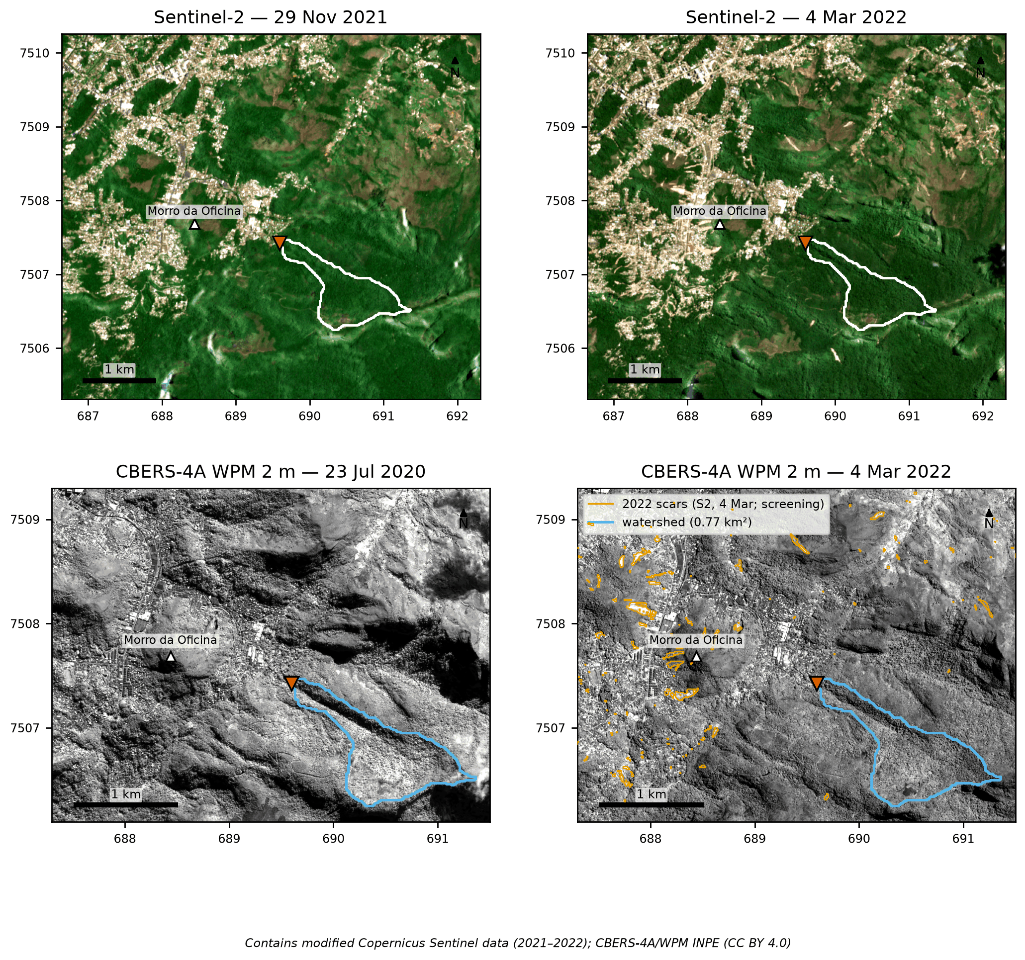
Figure 8.1: Images before and after the event. Top: Sentinel-2 L2A natural color, November 29, 2021 and March 4, 2022 (calibration window PET_calibracao_2022). Bottom: CBERS-4A/WPM 2-m panchromatic, July 23, 2020 and March 4, 2022, with the Sentinel-2 candidate polygons of exposed soil (orange). Contains modified Copernicus Sentinel data (2021–2022); CBERS-4A/INPE (CC BY 4.0).

8.2 Siting the Sabo dam and defining the reference point

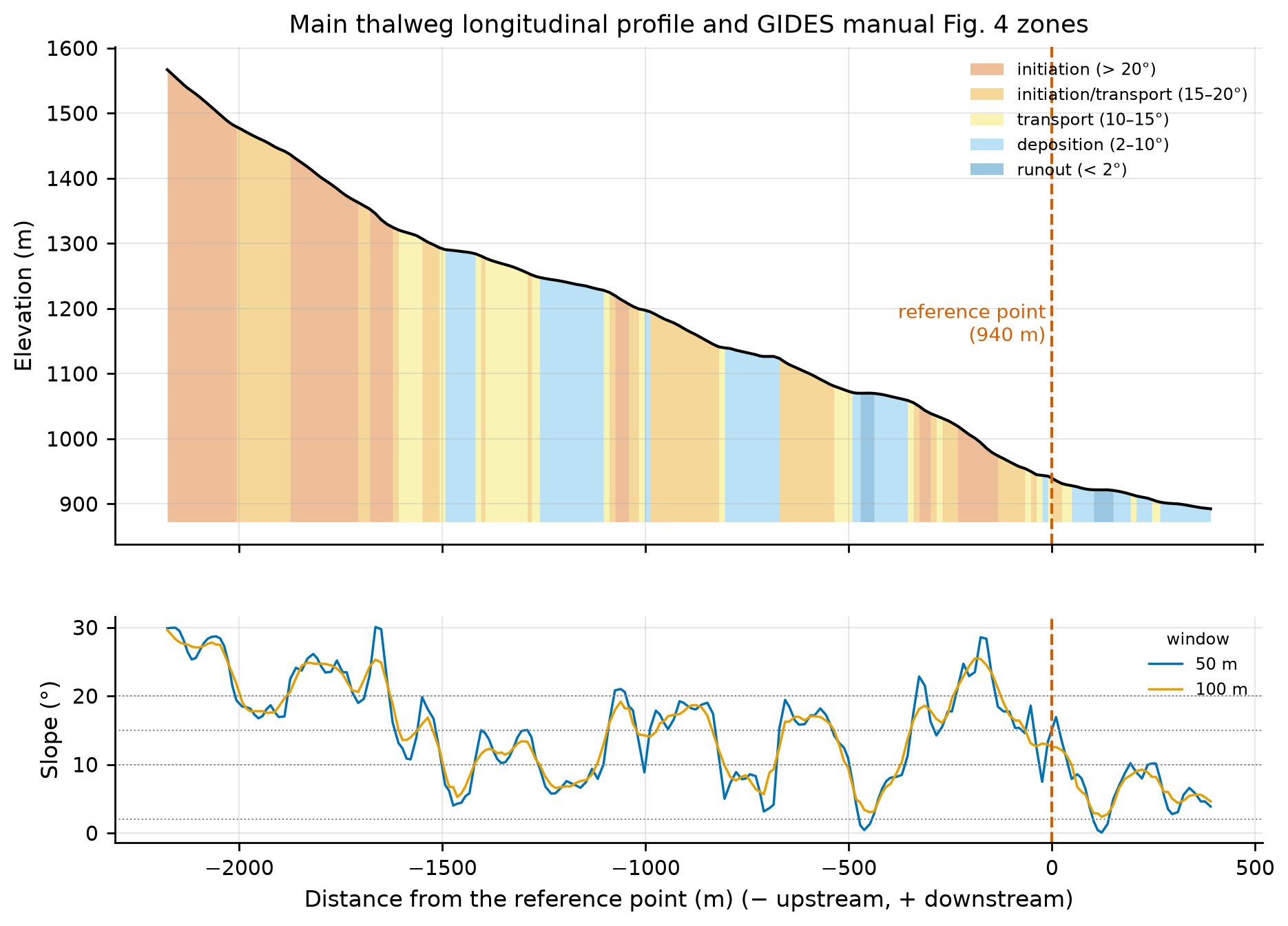
The GIDES manual (§2.4; Fig. 4) places the reference point downstream of the transport zone and upstream of the area to be protected; in Japanese practice (NILIM TN 904, §2.4 — NILIM: Japan’s National Institute for Land and Infrastructure Management), it is the valley outlet immediately upstream of the assets to be protected, that is, the downstream end of the transport reach. The zones by channel-bed slope are: > 20° initiation; 15–20° initiation/transport; 10–15° transport; 2–10° deposition; < 2° runout.

The coordinate provided fell on a hillslope with only 0.4 ha of contributing area, 40–75 m east of a 0.77-km² channel that runs from the southeast (1,567 m) to the northwest and enters Alto da Serra. The systematic search of project step 10 evaluated five candidates (Table 8.2).

Table 8.2: Reference-point candidates (SIRGAS 2000/UTM 23S; ANADEM 10 m). Source: bacia/caso.json and docs/pesquisa/10_locacao_bacias.md.

Id	Description	E / N (m)	Elevation	Area	Slope 50 m / 200 m upstr. / 100 m downstr.	1st building downstream
A (final)	valley outlet next to the point provided	689,595 / 7,507,425	940 m	0.77 km²	15.1° / 18.0° / 9.8°	72 m
B	western tributary	689,445 / 7,507,415	928 m	0.45 km²	15.1° / 15.2° / 9.5°	0 m (inside the built-up area)
C	main branch above the 1,070-m bench	690,025 / 7,507,135	1,087 m	0.66 km²	17.2° / 13.1° / 8.8°	628 m
D	northern valley	689,775 / 7,507,735	941 m	2.13 km²	12.8° / 13.6° / 9.4°	0 m
E	valley with NDVI loss in 2022	688,975 / 7,508,955	931 m	0.38 km²	13.9° / 13.1° / 9.4°	114 m

Choice: A (Table 8.3). It is the valley outlet immediately upstream of the first houses (72 m), with a forested watershed and no buildings. The local slope is still 15.1° — at the lower limit of the initiation/transport class (15–20°) — and deposition (< 10°) only begins about 48 m downstream, already next to the houses: there is no free deposition reach between the valley and the built-up area, so the rule “upstream of the area to be protected” prevails. B and D start inside the built-up area; C would leave 630 m of valley unprotected; E lies 1.7 km outside the indicated area.

Table 8.3: Rationale for the Petrópolis reference point (decision D15).

Item	Value
Coordinate provided	22°31’46.85”S, 43°09’21.52”W → 689,650 E / 7,507,373 N (956 m; hillslope)
Final point	689,595 E / 7,507,425 N; −22.529220, −43.156517 (22°31’45.19”S, 43°09’23.46”W)
Shift	75 m
Elevation (ANADEM)	939.5 m (≈ 940 m)
Bed slope: local (50 m) / mean over 200 m upstream / 100 m downstream	15.1° / 18.0° / 9.8°
Zone (Fig. 4 of the manual)	downstream end of the transport reach (15.1°, lower limit of the 15–20° class); deposition (< 10°) from ~48 m
Protected area	Alto da Serra/Morin: 1st building at 72 m; 48 OSM buildings in the 50 m × 500 m corridor; Ronaldo Silveira, Locarno, Lucerne, Saint Moritz, Dr. Públio de Oliveira, and Anésio de Oliveira streets
Cross section at the point	W1 = 36 m, W5 = 64 m, W10 = 86 m (width up to 1, 5, and 10 m above the valley floor)

The longitudinal profile (Figure 8.2) is stepped, with benches at ~1,070 m and ~1,130 m that alternate deposition and initiation reaches along the valley — a pattern typical of the stepped bedrock channels of the Serra do Mar. At the point, the slope over a 50-m window is 15.1°; downstream, it passes through 16.9° (10 m) and 11.2° (34 m) and only drops below 10° at 48 m (bacia/perfil_longitudinal.csv).

Figure 8.2: Longitudinal profile of the main thalweg (2,177 m, from the divide at 1,567 m to the point at 940 m, plus 400 m downstream) with the zones of Fig. 4 of the GIDES manual based on the slope over a 50-m window. Bottom: slope over 50-m and 100-m windows.

8.3 Input datasets

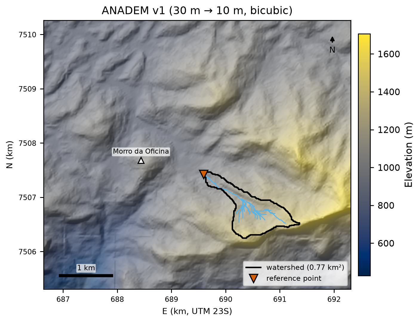
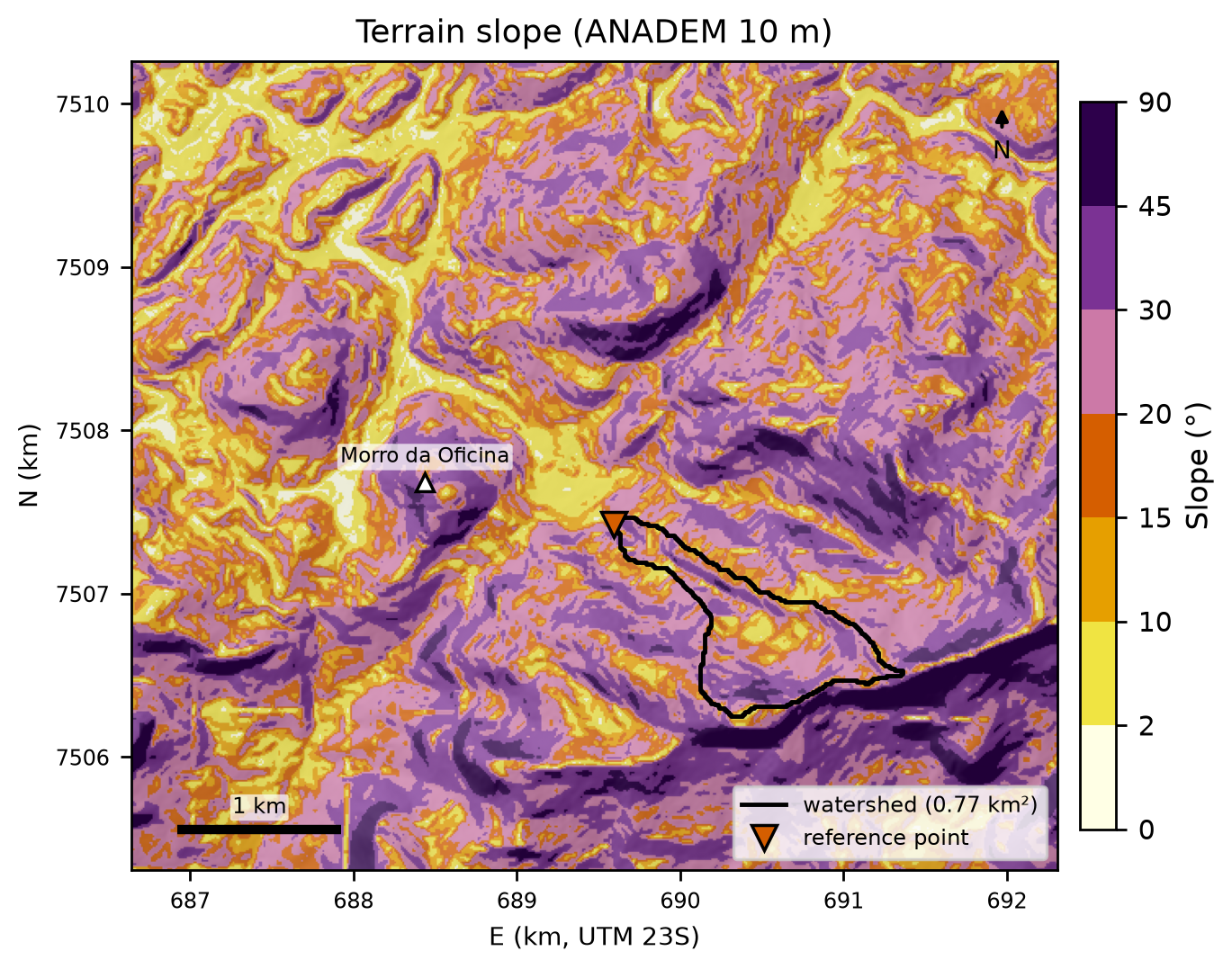
Table 8.4 summarizes the datasets used. All of them were standardized to SIRGAS 2000/UTM 23S (EPSG:31983) in project step 05 and are shown here over the calibration window PET_calibracao_2022 (5.67 × 4.95 km), which contains the watershed (black outline), Alto da Serra, and Morro da Oficina (white triangle).

Table 8.4: Input datasets of the Petrópolis case (IBGE: Brazilian Institute of Geography and Statistics; SGB: Geological Survey of Brazil; UERJ: Rio de Janeiro State University). Details, URLs, and SHA-256 checksums in data/raw/*/FONTE.md and docs/pesquisa/05_bases.md.

Layer	Source	Resolution/scale	Date	License
DEM and shaded relief	ANADEM v1 (Laipelt et al., 2024)	30 m (resampled to 10 m, bicubic)	—	CC BY 4.0
Slope and D8 flow direction	derived from the 10-m ANADEM (pysheds)	10 m	—	—
Soils	IBGE BDiA Pedology	1:250,000	RADAMBRASIL compilation; 2021 legend	free use with attribution
Geology	SGB/UERJ geological map sheets	1:100,000	—	SGB public data
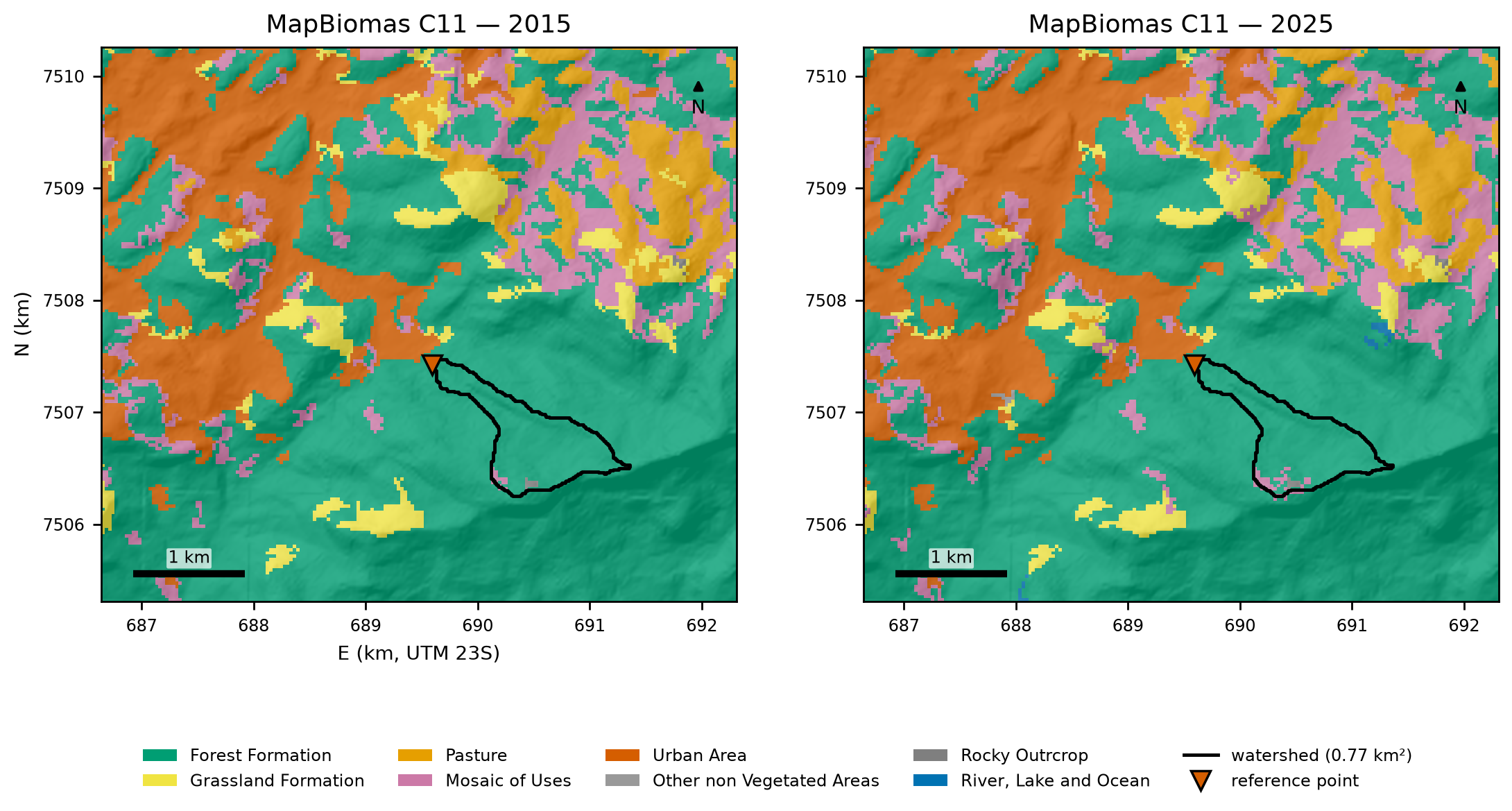
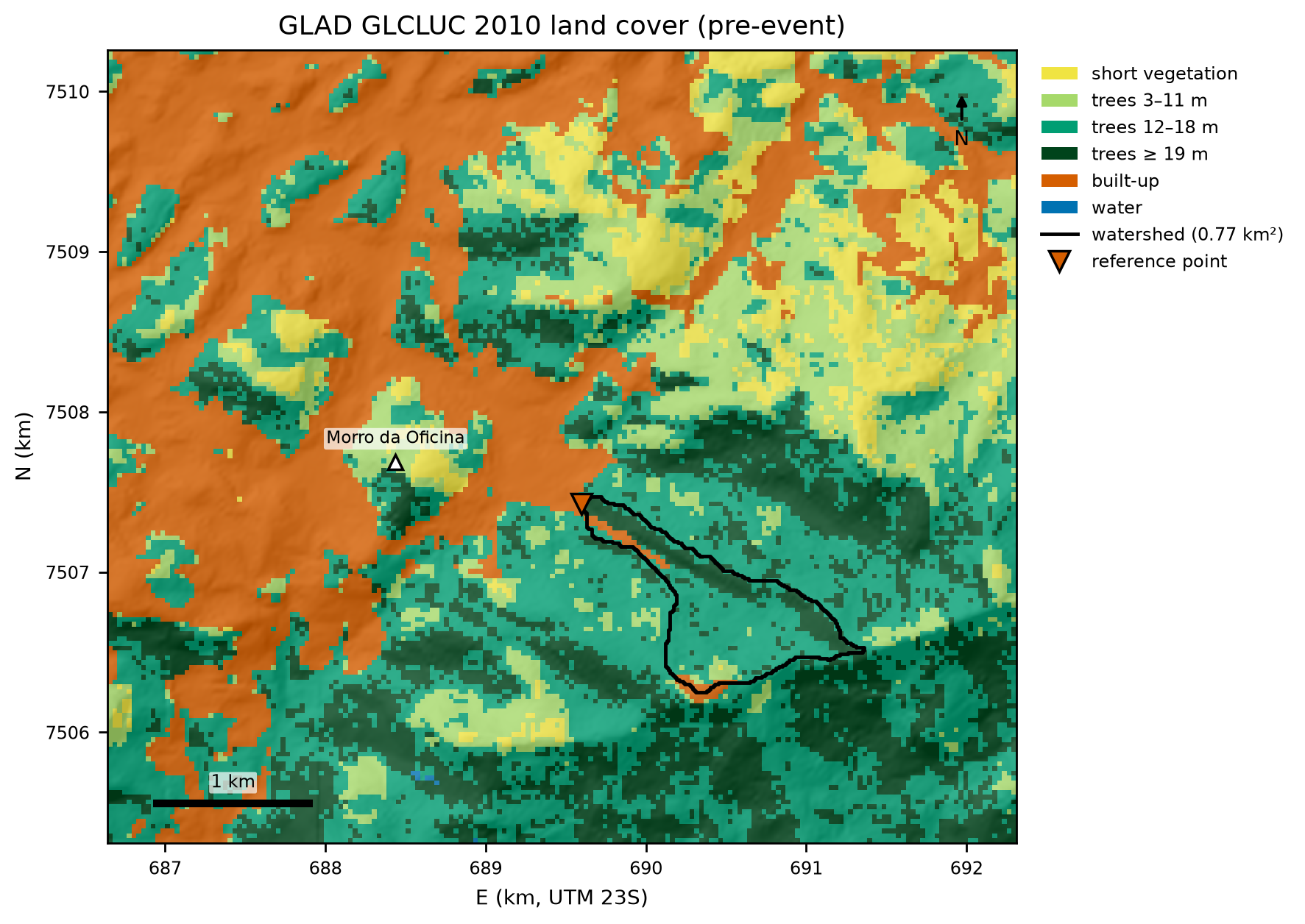
Land cover (before the 2011 event)	GLAD GLCLUC 2010 (Potapov et al., 2022)	30 m	2010	CC BY
Land cover	MapBiomas Collection 11	30 m	2015 and 2025	CC BY 4.0
Soil texture	ISRIC SoilGrids 2.0 (Poggio et al., 2021)	250 m	—	CC BY 4.0
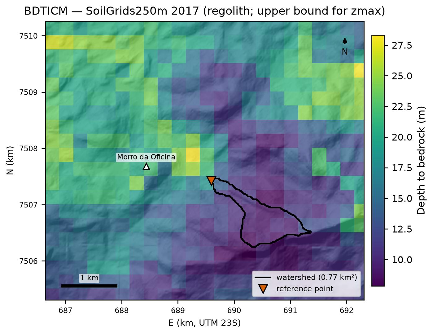
Depth to bedrock	SoilGrids250m 2017, BDTICM (Shangguan et al., 2017)	250 m	2017	ODbL
Imagery	Sentinel-2 L2A (Copernicus; Planetary Computer) and CBERS-4A/WPM (INPE)	10 m and 2 m	2020–2022	Copernicus terms; CC BY 4.0
Buildings and roads	OpenStreetMap	vector	Oct 30–31, 2026	ODbL

8.3.1 Relief, slope, and flow direction

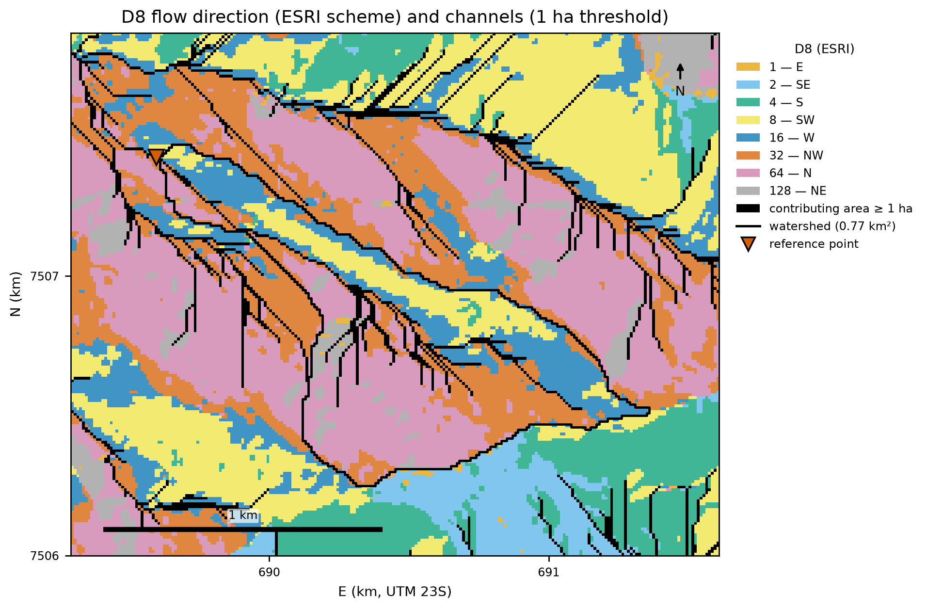
ANADEM is a digital terrain model (vegetation removed from Copernicus GLO-30). The watershed ranges from 940 m to 1,567 m (Figure 8.3), with a mean slope of 24.5° and 30% of its area steeper than 30° (Figure 8.4). The D8 flow direction (Figure 8.5) shows the well-known D8 artifact on planar slopes: parallel flow lines, which inflate the number of channel heads (Section 8.4).

Figure 8.3: ANADEM DEM (10 m) with shaded relief and the watershed’s drainage network.

Figure 8.4: Terrain slope in classes that include the limits of Fig. 4 of the GIDES manual (2°, 10°, 15°, and 20°).

Figure 8.5: D8 flow direction (ESRI scheme: 1 = east … 128 = northeast) and cells with contributing area ≥ 1 ha.

8.3.2 Soils, texture, and geology

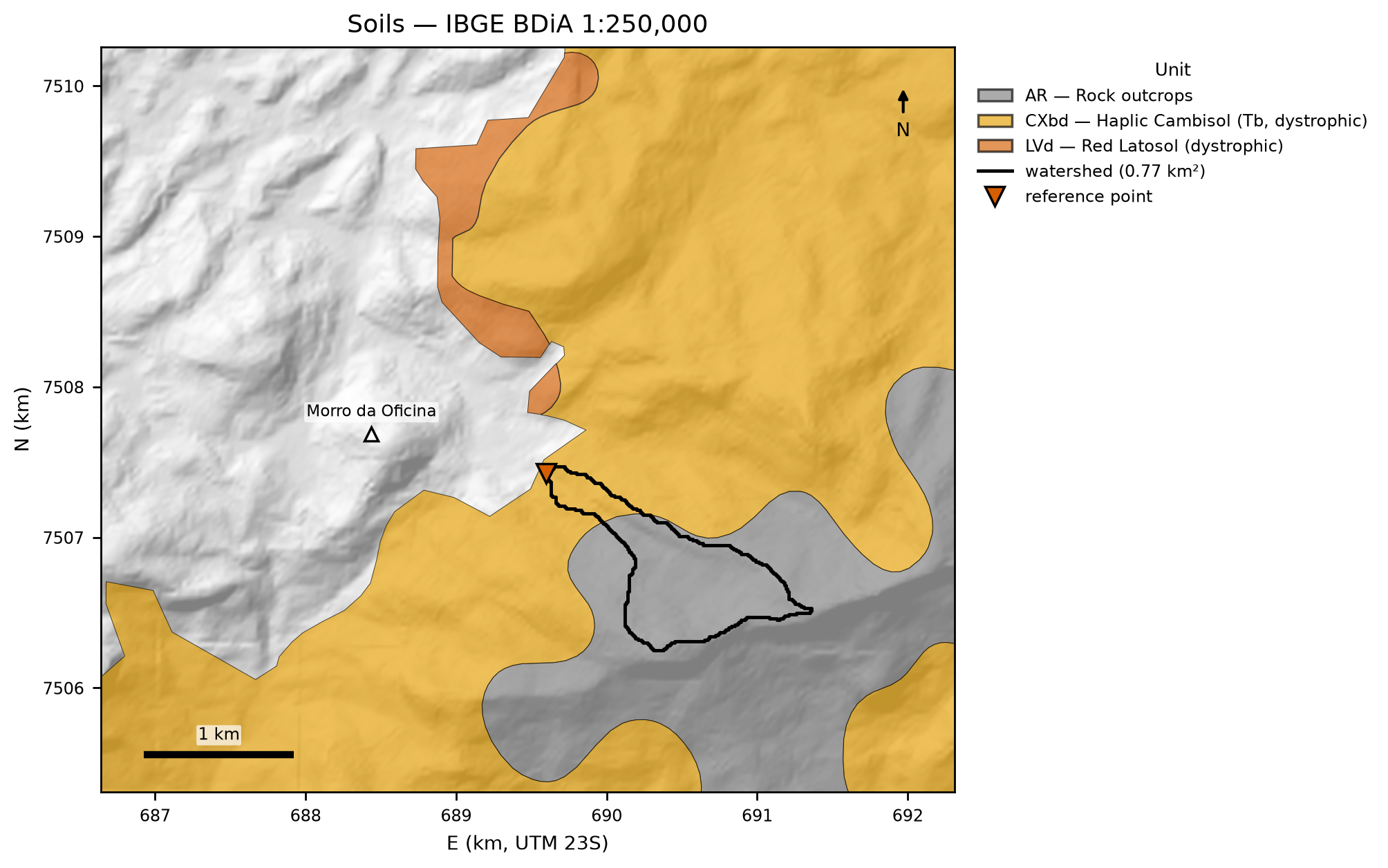
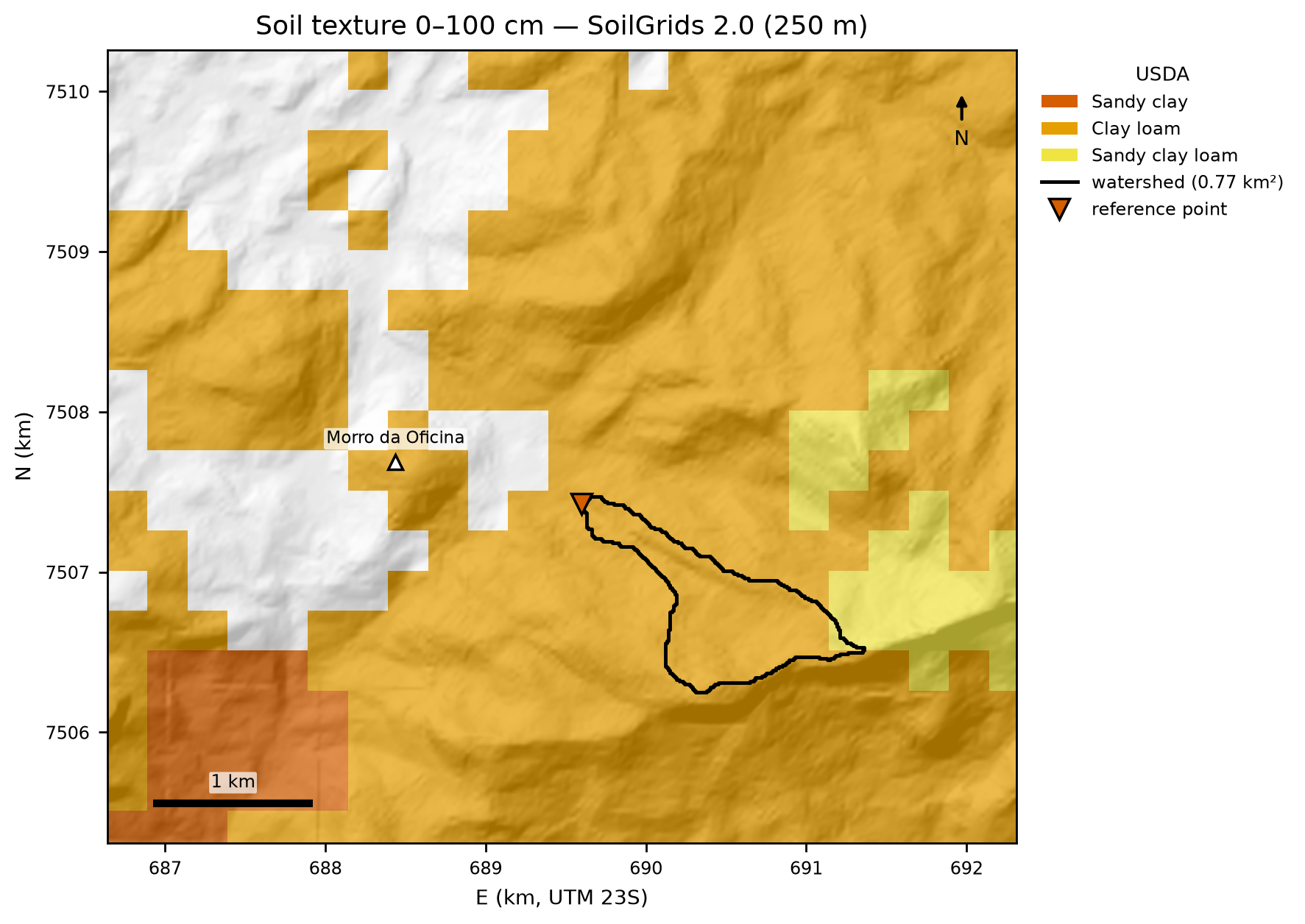
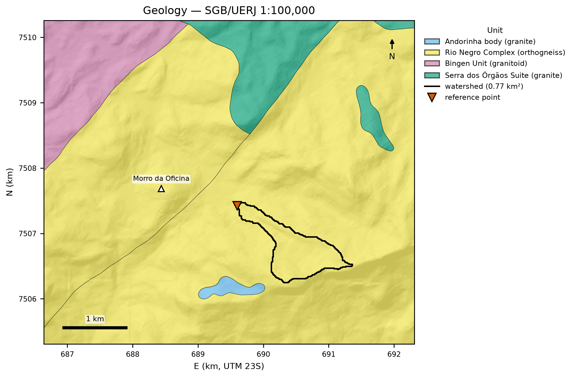
On the 1:250,000 soil map, 86% of the watershed — its entire upstream part — lies in unit AR3: rock outcrops as the dominant component, associated with Haplic Cambisol (Tb, dystrophic) and Litholic Neosols (mountainous and steep relief), with inclusions of Red Latosol. Only 14%, in the downstream reach next to the outlet, lies in unit CXbd32 — Haplic Cambisol (Tb, dystrophic; Cambissolo Háplico Tb Distrófico in the Brazilian soil classification), with humic Yellow and Red-Yellow Latosols and inclusions of Litholic Neosols and Humic Cambisol (Figure 8.6; areas in chuva/cn.json). The window also contains the dystrophic Red Latosol (LVd3) and a patch mapped as urban area, with no soil unit. SoilGrids 2.0 classifies 22 of the watershed’s 25 pixels (250 m) as clay loam and 3 as sandy clay loam, with a 0–100 cm weighted mean of 41.7% sand, 26.5% silt, and 31.8% clay (Figure 8.7). The 1:100,000 geology places the entire watershed in the Rio Negro Complex (orthogneisses, metadiorites, tonalites, and leucogranites; Figure 8.8).

Figure 8.6: Soils — IBGE BDiA 1:250,000.

Figure 8.7: USDA texture class (0–100 cm weighted mean) — SoilGrids 2.0.

Figure 8.8: Geology — SGB/UERJ 1:100,000 map sheets.

8.3.3 Land use and land cover

The watershed is almost entirely forest: 97.1% in 2015 and 94.1% in 2025 according to MapBiomas, with 1.2% rock outcrop and the remainder in a mosaic of uses (Figure 8.9). GLAD 2010 — used as the pre-2011 state, because MapBiomas 2010 could not be obtained — indicates a canopy with a median height of 17 m (P25–P75: 17–20 m) in the watershed (Figure 8.10). The urban area of Alto da Serra begins 72 m downstream of the reference point.

Figure 8.9: Land cover and use — MapBiomas Collection 11, 2015 and 2025.

Figure 8.10: GLAD GLCLUC 2010 land cover with tree-height classes.

8.3.4 Depth to bedrock, zones, and initial water table

The SoilGrids250m 2017 BDTICM layer gives 7.9–14.1 m (median 9.9 m) in the watershed (Figure 8.11). This value represents the regolith/saprolite, not the soil thickness that can be mobilized by shallow landslides (0.5–2 m in the Serra do Mar; docs/pesquisa/04_parametros_trigrs.md). For this reason it is used neither as a thickness nor as a cap: it always lies above the general 5-m cap of the zmax grid and enters only as a rescaled spatial pattern in the alternative “regolith” model of the sensitivity analysis. The effective bedrock cap is given by the caps of each geotechnical unit (0.1 m on the outcrop; 0.5 and 1.0 m in the shallow soil over rock). The grids of property zones, zmax, and initial water table (scenarios from 1 to 10 m capped at the bedrock contact, depthwt = min(d, zmax), decision D6) are produced in the TRIGRS parameterization and presented in Section 8.8.

Figure 8.11: Depth to bedrock (BDTICM, SoilGrids250m 2017).

8.4 Watershed delineation and drainage network

The procedure is the same as in the Nova Friburgo chapter, using the code of project step 10 (docs/pesquisa/10_locacao_bacias_codigo/):

1. DEM: ANADEM reprojected to EPSG:31983 at 30 m (bilinear) and 10 m (bicubic), both from the original.
2. Conditioning: fill_pits → fill_depressions → resolve_flats (Barnes et al., 2014) in pysheds; within the watershed, filling changed 10 cells, by at most 1.31 m.
3. D8 direction (ESRI scheme) and flow accumulation (O’Callaghan & Mark, 1984).
4. Channel initiation: the manual’s criterion (a = b on the contour lines) is not resolved by a 30-m DEM (maximum b/a of 0.75 along the thalweg). A 1-ha threshold of contributing area was adopted, calibrated on Appendix A of the manual (Nova Friburgo).
5. Strahler order (Strahler, 1957) and zero-order thalwegs: from the channel heads up to the divide, plus convergent lateral hollows (A ≥ 0.25 ha and effective width ≥ 30 m).

Table 8.5: Metrics of the Petrópolis watershed (bacia/caso.json).

Metric	Value (10 m)	Value (30 m)
Area A	0.7712 km²	0.7785 km²
Perimeter; compactness Kc; form factor Kf	6.16 km; 1.96; 0.163	6.12 km
Minimum / mean / maximum elevation	939.5 / 1,282.5 / 1,567.3 m	—
Mean watershed slope	24.5° (47.8%); 30% of the area > 30°	—
Main thalweg L; slope S	2,177 m; 0.288 m/m (16.1°)	2,095 m
tc Kirpich / Giandotti / Ven Te Chow	11.7 / 27.5 / 23.6 min	11.4 / 27.4 / 23.0 min
Channel heads; maximum order	25; 4	26; 4
Ldy11 (orders 1 to 4)	5,769 m (3,553 / 816 / 514 / 886 m)	6,847 m
Ldy12 (zero order; headwater + lateral)	10,397 m (8,233 + 2,164 m; 36 thalwegs)	11,646 m
Drainage density	7.48 km/km²	8.80 km/km²
Bd(DEM), valley-floor width up to 1 m above the bed (34 sections)	median 28 m (P25–P75: 21–43 m)	—

Figure 8.12: Watershed, Strahler network (1-ha threshold), zero-order thalwegs, buildings (OSM), and 2022 scar candidates (Sentinel-2, March 4, 2022: filled = base rule; outline = calibrated rule).

WarningChannel length depends on the threshold

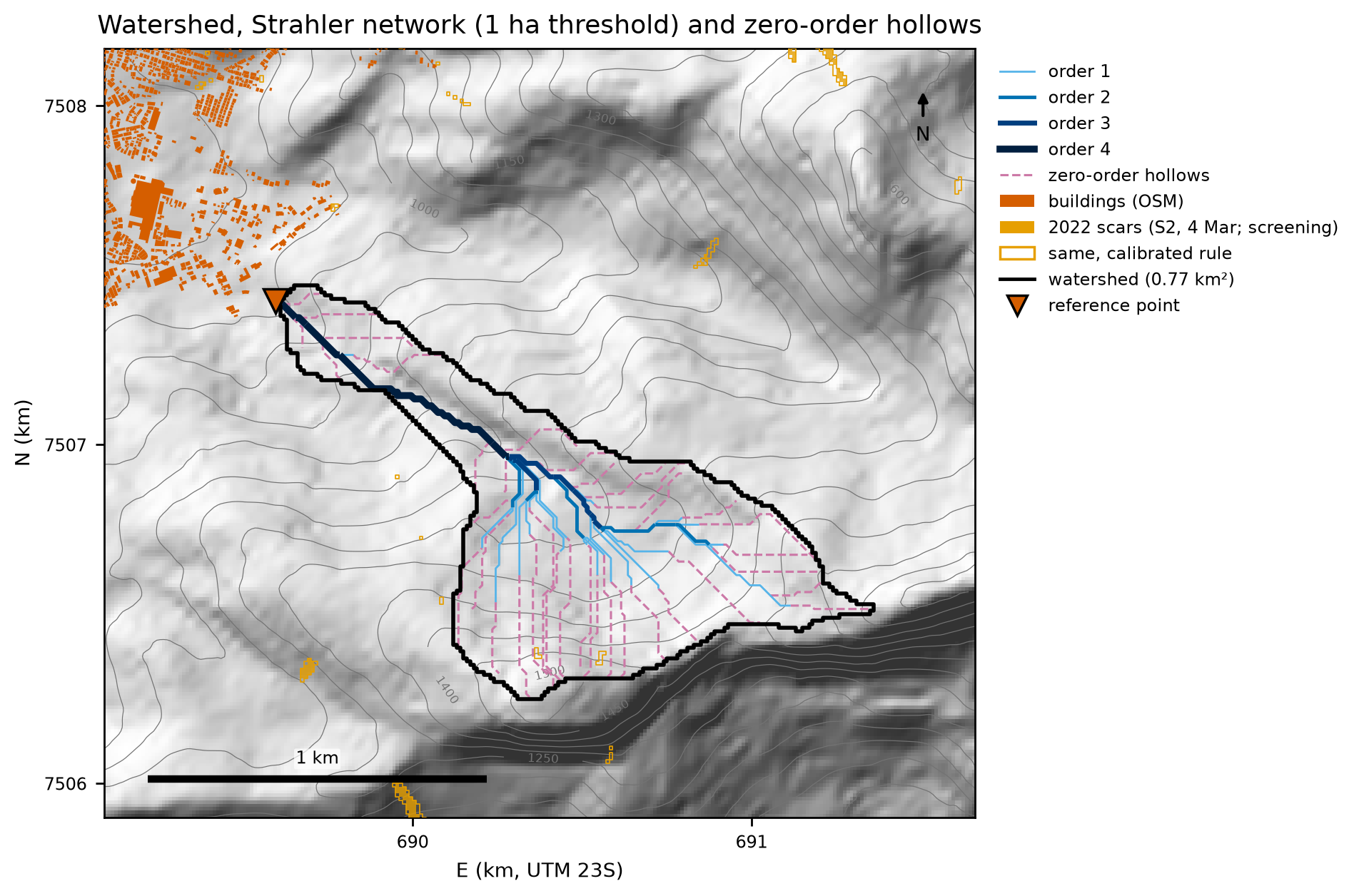
Between 1 and 5 ha, Ldy11 drops from 5,769 to 1,976 m and Ldy12 from 10,397 to 8,209 m (gides/tabelas/sensibilidade_limiar_canal.csv): length shifts from order ≥ 1 to order zero. Since GIDES method “b” multiplies these lengths by an erodible cross section, the threshold is a volume parameter and enters the sensitivity analysis of Section 8.7.

8.5 Design rainfall

TipCompanion scripts for this section

cd /Projetos/trigrs-mapper/scripts/casos/petropolis
PY=/Projetos/trigrs-mapper/.venv/bin/python
$PY 01_chuva_frequencia.py      # stations, annual maxima, frequency, Pd(TR), regional
$PY 02_idf_hietogramas_clima.py # IDF, design hyetographs, climate factors
$PY 03_cn_hidrograma.py         # CN (DPM database, BHAE 2022), SCS-CN, UH and hydrographs
$PY 04_eventos.py               # Feb 15 and Mar 20, 2022 hyetographs and antecedent rainfall

8.5.1 Rain gauges and selection

Under the rules of the project’s rainfall report (docs/pesquisa/06_chuva.md), candidate stations need ≥ 30 valid years, recent data, proximity, and an orographic position similar to that of the watershed. In Petrópolis no station meets all of these requirements, so we work with a reference trio plus an older complementary series (Table 8.6, Figure 8.13). The Cemaden/INEA rain gauges that recorded the 2022 event have only ~45 days from 2015 in the database of the DPM (Department of Disaster Prevention and Mitigation of SEDEC/MIDR — Brazil’s National Secretariat of Civil Protection and Defense, Ministry of Integration and Regional Development) and are of no use for frequency analysis.

Table 8.6: Stations used in the frequency analysis (chuva/estacoes.csv; INMET: National Institute of Meteorology).

Code	Station (operator)	Lat; lon	Elev. (m)	Dist. to point (km)	Period in database	Valid years (used)	Role
02243009	Petrópolis (ANA)	−22.5117; −43.1708	890	2.4	1938–2007	58 (58; 1939–2004)	design station
02243010	Itamarati-SE (ANA/SGB-CPRM)	−22.4853; −43.1492	1,085	4.9	1938–Jan 2026	87 (85; 1939–2025)	reference
02243011	Rio da Cidade (ANA/SGB-CPRM)	−22.4381; −43.1703	704	10.2	1938–Feb 2026	85 (85; 1939–2025)	reference
02243188	Petrópolis — Parque Nacional (INMET)	−22.5333; −43.1833	895	2.8	1912–1959	35 (35; 1922–1959)	complementary
02243001	Andorinhas (ANA)	−22.5333; −43.0500	210	11.0	1947–1996	29 (28)	informative (n < 30)

Figure 8.13: Rain-gauge stations, regional relief (ANADEM), and the position of the watershed. The white square is the INEA Alto da Serra gauge, used to reconstruct the event (Section 8.5.7).

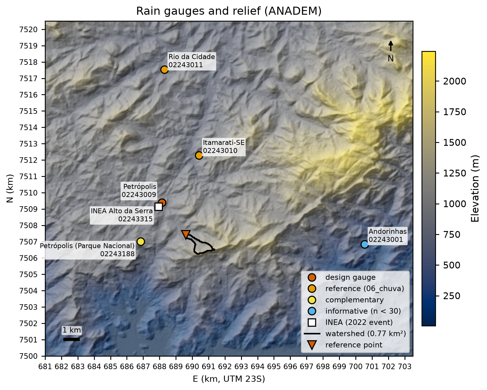
The design station is 02243009 Petrópolis: it is the closest one with ≥ 30 years and has the same orographic position as the watershed — the plateau immediately behind the Serra do Mar escarpment, at about 900 m. The current series (Itamarati-SE and Rio da Cidade) lie 5–10 km to the north, on the inland (lee) side of the range, and have smaller extremes (means of the annual maxima of 90.2 and 84.7 mm versus 104.2 mm). The design series ends in 2007; the stationarity assumption is supported by the absence of a significant trend in the maxima of all stations (Mann–Kendall, Table 8.7). Andorinhas, at the windward foot of the escarpment, is used only as context: it has 29 valid years and the highest reading in the region (395.4 mm on December 3, 1981).

8.5.2 Annual-maximum series and quality control

We use the annual maximum 1-day rainfall (7 a.m. reading, ANA’s HIDRO database) in the calendar year, as in the GIDES manual, and the water year (Oct–Sep) as a sensitivity case. A year is accepted if it has ≤ 10% of days missing; maxima flagged with ANA status 3 (doubtful) or 4 (accumulated) are excluded — as for Itamarati-SE in 2023 (58.0 mm) and 2024 (96.0 mm). Figure 8.14 shows the series and Table 8.7 the tests.

Figure 8.14: Annual maximum daily rainfall at the stations (calendar year). The asterisk marks the published February 15, 2022 value at São Sebastião (Cemaden, 24 h), which is not a reading of station 02243009, closed in 2007.

Table 8.7: Statistics and quality tests (calendar year). Grubbs–Beck per Bulletin 17B (IACWD, 1982); r₁ limits from Anderson (1942).

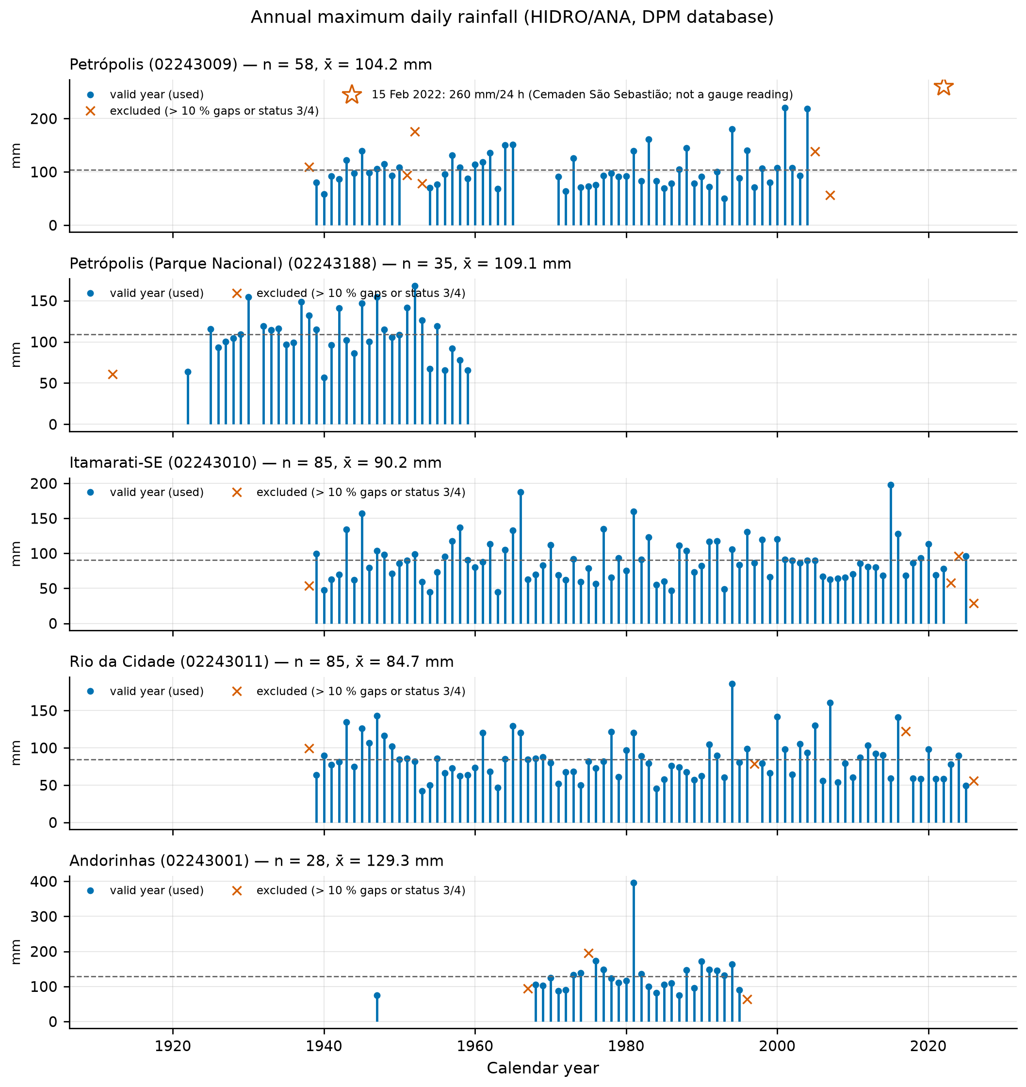
Station	n	x̄ (mm)	s (mm)	g	Grubbs–Beck (10%)	r1 (independence, 95%)	Mann–Kendall: p; Sen (mm/yr)
02243009 Petrópolis	58	104.18	35.06	1.43	no outliers (upper limit 235.9 mm)	−0.12 (ok)	0.49; +0.17
02243010 Itamarati-SE	85	90.19	30.17	1.17	no outliers	−0.02 (ok)	0.91; +0.01
02243011 Rio da Cidade	85	84.74	28.03	1.10	no outliers	−0.005 (ok)	0.37; −0.10
02243188 Parque Nacional	35	109.09	28.09	0.09	no outliers	0.14 (ok)	0.78; −0.20
02243001 Andorinhas	28	129.32	59.28	3.50	395.4 mm above the limit (282.8 mm)	0.05 (ok)	0.28; +1.01

The highest readings at the design station are 220.1 mm (December 24, 2001) and 218.2 mm (December 21, 2004); on February 6, 1988 — the disaster with 171 deaths — it recorded 145.0 mm.

8.5.3 Frequency analysis and Pd(TR)

To obtain Pd(TR), the design 1-day rainfall for return period TR, we fitted seven distributions to the design series by three methods (moments, L-moments, and maximum likelihood), with goodness-of-fit tests (Kolmogorov–Smirnov, Anderson–Darling, chi-square, and PPCC; p-values by parametric bootstrap for the L-moment fits), AIC/BIC, and the L-moment ratio diagram (Hosking & Wallis, 1997). Two criteria are shown side by side:

• GIDES manual criterion (Appendix A): skewness g = 1.43 < 1.5 → Gumbel by the method of moments, with α = 0.779·s = 27.32 mm and β = x̄ − 0.577·α = 88.42 mm. The manual only gives the threshold rule; the script records the warning that g is close to it (the choice is sensitive to the sample; chuva/ajustes.json).
• Modern criterion (rule recorded in the script): the 3-parameter distribution closest to the sample on the L-moment ratio diagram, estimated by L-moments, provided it is not rejected by the goodness-of-fit tests and has ΔAIC ≤ 2. The sample (τ₃ = 0.253; τ₄ = 0.192) lies practically on the GEV curve (distance 0.003).

Table 8.8: Fits to the 02243009 series (n = 58). KS and AD p-values by parametric bootstrap (300 simulations) for the moment (manual) and L-moment fits; “—” = not computed. All fits in chuva/ajustes.json.

Distribution / method	AIC	KS: D; p	AD: A²; p	PPCC r	P100 (mm)	P200 (mm)
Gumbel — manual’s moments	563.6	0.087; 0.42	0.41; 0.50	0.987	214.1	233.1
Gumbel — ML	562.5	0.073; —	0.31; —	0.987	203.0	220.2
GEV — L-moments (chosen)	563.5	0.062; 0.68	0.17; 0.86	0.993	233.3	263.7
GEV — ML	563.4	0.060; —	0.18; —	0.992	225.7	252.3
LN3 — L-moments	565.0	0.068; 0.57	0.21; 0.70	0.993	229.3	255.8
LP3 — ML	563.6	0.065; —	0.20; —	0.992	221.3	245.6
LN2 — ML	563.8	0.091; —	0.43; —	0.983	201.3	217.1

The candidates in the table pass the goodness-of-fit tests, and the (ML) AICs of Gumbel, GEV, LP3, LN3, and LN2 differ by less than 1.3 units (Pearson III: 2.2; the 2-parameter exponential fitted by ML is rejected by KS) — the 58-year sample does not discriminate between the tails. The choice falls on the GEV fitted by L-moments (ξ = 87.34 mm, α = 23.48 mm, k = −0.125, heavy tail) for three reasons: (i) it is the distribution indicated by the L-moment ratio diagram, the most robust diagnostic for short hydrological series (Hosking & Wallis, 1997); (ii) the two highest readings (2001 and 2004) lie well above the Gumbel curve (Figure 8.15), and the global literature shows that daily rainfall maxima usually have heavier tails than the Gumbel (Papalexiou & Koutsoyiannis, 2013); (iii) for a structure that protects lives, the conservative choice is preferable. The manual’s Gumbel is kept for comparison and as the lower bound of the range.

Figure 8.15: Gumbel probability paper. (a) Design station: sample (Gringorten plotting positions), fits, and 90% CI (bootstrap) of the GEV-L; the dashed line is the February 15, 2022 value converted to 1 day. (b) Fits chosen at each station of the trio and at the complementary station.

NoteRegional check (index flood)

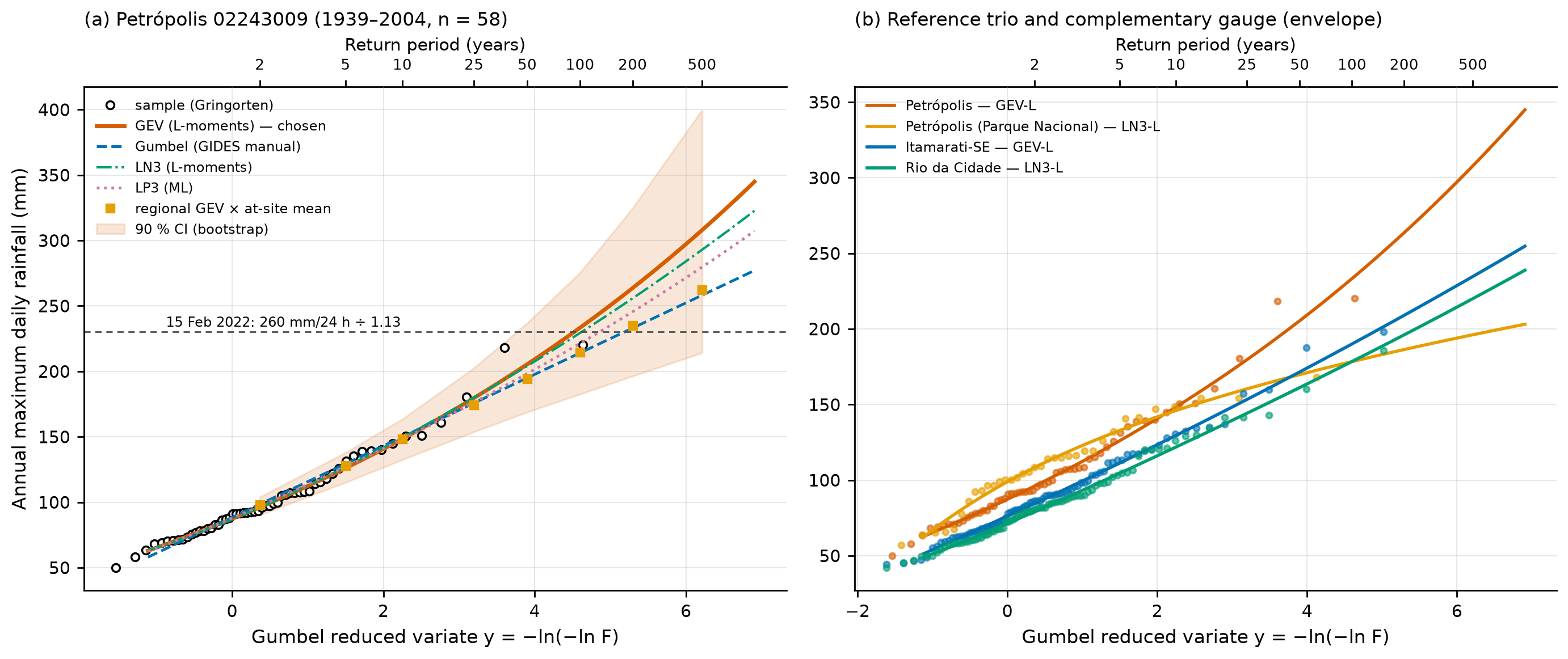
With the four stations that have n ≥ 30, the weighted L-moment ratios are τ_R = 0.176, τ_3R = 0.187, and τ_4R = 0.160, and the heterogeneity measure H1 = −0.36 (500 kappa simulations) classifies the region as acceptably homogeneous (Hosking & Wallis, 1997). The regional GEV growth curve multiplied by the local mean (104.18 mm) gives P100 = 214.5 mm and P200 = 235.0 mm — practically the manual’s Gumbel (chuva/regional_lmom.json). The difference from the local GEV comes from τ₃: 0.253 at 02243009 and only 0.023 at the neighboring Parque Nacional station (1922–1959), two gauges 2.7 km apart. With only four gauges the H1 test has little power; the regional result is kept as a check, within the 90% CI of the local estimate.

The 90% CI comes from 2,000 nonparametric bootstrap replicates, refitting the GEV by L-moments in each replicate. Table 8.9 gives the adopted Pd(TR); TR > 3n = 174 years is an extrapolation.

Table 8.9: Design maximum 1-day rainfall Pd(TR) and comparisons (chuva/pd_tr.csv).

TR (years)	2	5	10	25	50	100	200	500
Adopted Pd (GEV-L), mm	96.1	126.1	148.4	179.7	205.4	233.3	263.7	307.9
90% CI, lower	90.3	115.1	132.5	153.8	168.8	182.6	196.4	214.1
90% CI, upper	104.0	137.9	163.5	202.6	237.0	275.4	324.7	399.8
Manual’s Gumbel	98.4	129.4	149.9	175.8	195.0	214.1	233.1	258.1
Regional GEV × local mean	98.1	128.0	148.3	174.5	194.4	214.5	235.0	262.5
Itamarati-SE (GEV-L)	84.6	111.3	129.6	153.4	171.6	190.1	209.0	234.7
Rio da Cidade (LN3-L)	79.2	104.6	121.9	144.2	161.2	178.5	196.1	220.1
Parque Nacional (LN3-L)	108.4	132.9	146.0	160.4	169.8	178.4	186.4	196.2

Figure 8.16: Adopted Pd(TR) with 90% CI, envelope of the stations (each with its chosen distribution), the manual’s Gumbel, the regional GEV, and reference values from other cases.

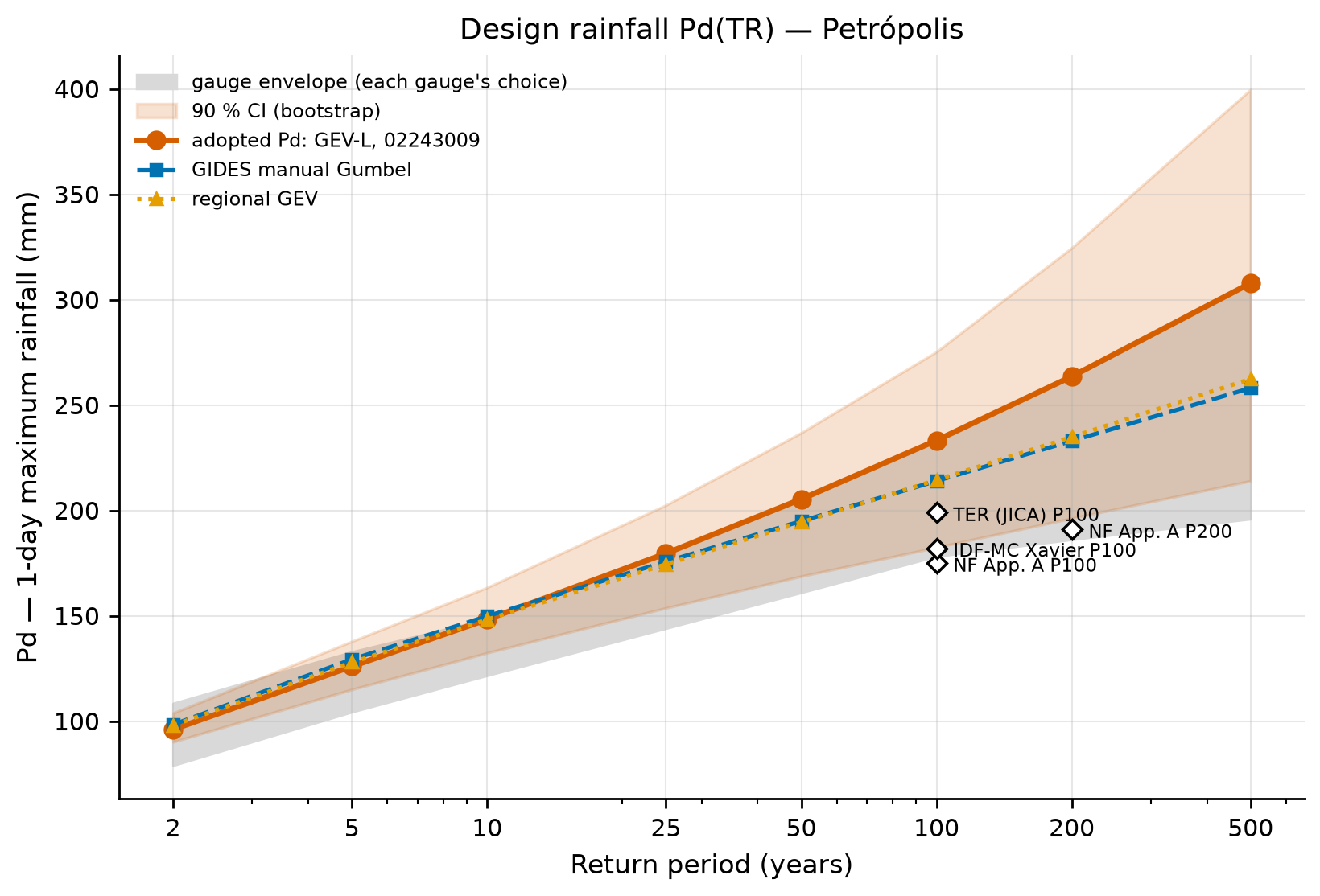
Comparison with other references. The Petrópolis P100 (233 mm) is 33% higher than that of the gauge used in Appendix A of the manual in Nova Friburgo (P100 = 175 mm, P200 = 191 mm), 17% higher than the P100 of the JICA/SABO project in Teresópolis (199 mm), and 28% higher than the gridded baseline of the IDF-MC Portal (SEDEC/MIDR’s IDF curves under climate change) for Petrópolis (182.1 mm, Xavier 1981–2024, which smooths extremes). This is consistent with the position of Petrópolis at the edge of the escarpment, where the orographic effect is strongest (Andorinhas, at the windward foot of the escarpment, reaches P100 ≈ 317 mm with the PE3-L, n = 28).

Sensitivities. The water year reduces the GEV-L P100 to 209.3 mm (−10%). With the calendar-year rule and the two doubtful Itamarati-SE maxima included, that station’s P100 goes from 190.1 to 188.9 mm.

ImportantWhat was the return period of the 2022 storm?

Converting the 24-h total to 1 day (÷ 1.13), the 260 mm at São Sebastião are equivalent to 230 mm/day: TR ≈ 93 years by the adopted GEV-L and ≈ 179 years by the manual’s Gumbel. The 223 mm at INEA Alto da Serra correspond to TR ≈ 40 years (GEV-L). In other words, the TR 100 design rainfall adopted here is of the same order as the event that killed more than 230 people — and the March 20, 2022 event (415 mm in 10 h) exceeds any plausible 1-day TR (TR > 1,000 years by the GEV-L), which underlines the importance of sub-daily durations and of multi-day accumulated rainfall.

scripts/casos/petropolis/01_chuva_frequencia.py (excerpt)

from trigrs_mapper.hydro import frequencia as FR

res = FR.analise_frequencia(x, anos=anos, trs=(2, 5, 10, 25, 50, 100, 200, 500, 1000))
gev = FR.ajustar_distribuicao(x, "gev", "lmom")          # chosen
ic = FR.intervalos_bootstrap(x, "gev", "lmom", trs=(2, 5, 10, 25, 50, 100, 200, 500),
                             n_boot=2000, nivel=0.90, seed=20261031)
print(res["criterio_manual"]["distribuicao"], gev.quantil(100))   # gumbel 233.3

8.5.4 IDF curves

The IDF relationship is derived from daily rainfall (there is no long recording-gauge series at the site):

1. 24 h from 1 day: \(P_{24h} = 1.13\,P_{1\,day}\) — the empirical factor of TP-40 (Hershfield, 1961), standard at the DPM and in the IDF-MC Portal; Weiss (1964) obtained ≈ 1.14 (8/7) theoretically, and DAEE/CETESB (1980; São Paulo State water and environmental agencies) adopt 1.14.
2. DAEE/CETESB (1980) cascade disaggregation: 1 h/24 h = 0.42; 30 min/1 h = 0.74; 5, 10, 15, 20, and 25 min over 30 min = 0.34, 0.54, 0.70, 0.81, and 0.91; 6, 8, 10, and 12 h over 24 h = 0.72, 0.78, 0.82, and 0.85.
3. Sherman equation fitted to the 96 points (8 TRs × 12 durations):

\[ i(t,T) = \frac{K\,T^{a}}{(t+b)^{c}} = \frac{1{,}060.42\,T^{0.2070}}{(t+11.84)^{0.7581}} \quad [\text{mm/h};\ t\ \text{in min};\ T\ \text{in years}] \tag{8.1}\]

with R² = 0.9973, RMSE = 5.29 mm/h, and a mean absolute percentage error of 3.2%; the monotonicity checks (i increases with T and decreases with t; depth increases with t) pass (chuva/idf.json). Table 8.10 gives the disaggregation for TR 100 and Figure 8.17 the curves.

Table 8.10: DAEE/CETESB disaggregation for TR = 100 years (P1day = 233.3 mm; P24h = 263.7 mm).

Duration	5 min	10 min	15 min	30 min	1 h	6 h	8 h	10 h	12 h	24 h
Depth (mm)	27.9	44.3	57.4	81.9	110.7	189.8	205.7	216.2	224.1	263.7
Intensity (mm/h)	334.3	265.5	229.4	163.9	110.7	31.6	25.7	21.6	18.7	11.0

Figure 8.17: Petrópolis IDF curves: DAEE/CETESB points and Sherman equation.

NoteThe 1-hour rainfall

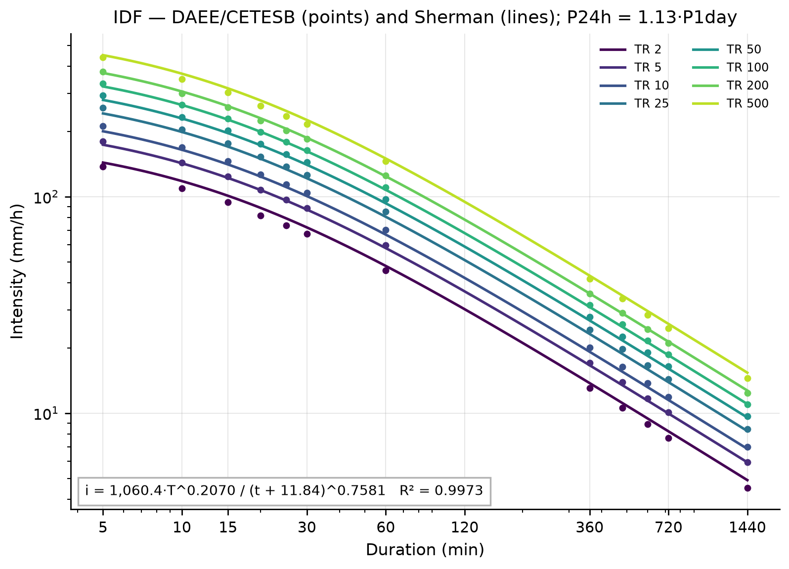
In the DAEE/CETESB cascade, the 1-hour rainfall (that of the wettest hour) is 0.42 × 1.13 = 47.5% of the 1-day rainfall: for TR 100, 110.7 mm/h, close to the hourly maximum measured on February 15, 2022 (103.4 mm/h). The SABO Manual Vol. 1 (SEDEC/JICA) cites, for the Serra do Mar, I₁ ≈ 0.28·Pp (Massad et al., 1997) — the choice of the 1 h/1 day ratio is a relevant uncertainty for TRIGRS, which responds to intensity.

8.5.5 Design hyetograph by the alternating block method

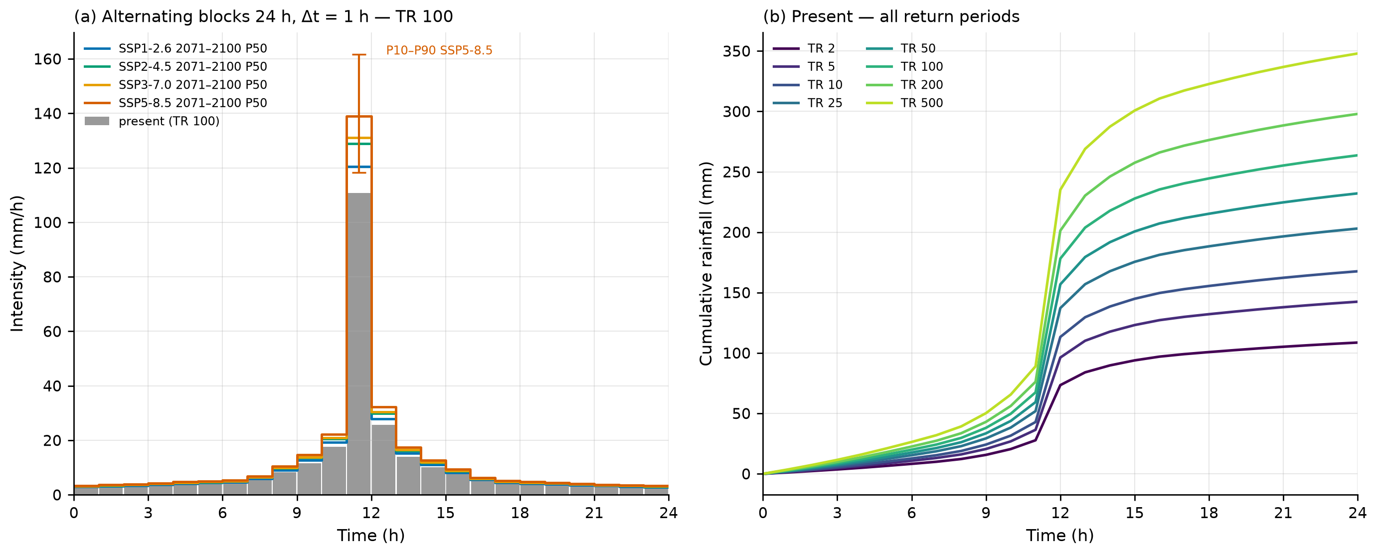
The 24-h hyetograph with a 1-h time step is built as follows (Chow, Maidment & Mays, 1988, §14.4):

1. For k = 1…24, \(P_k = P(k\,\Delta t)\) from the DAEE/CETESB depth–duration relationship (log-log interpolation between the nodes, exact at the nodes).
2. Increments \(\Delta P_k = P_k - P_{k-1}\), sorted from largest to smallest.
3. The largest goes to the central block (11–12 h); the following ones alternate to the right and to the left.

For TR 100: P(1 h) = 110.7 mm, P(2 h) = 136.4 mm, P(3 h) = 154.1 mm … P(24 h) = 263.7 mm; the increments are 110.7, 25.7, 17.7, 13.9, 11.7 … mm. The result is shown in Table 8.11 and Figure 8.18.

Table 8.11: TR 100 design hyetograph, present climate (total 263.7 mm). For TRIGRS: cri (m/s) = mm/h ÷ 3.6×10⁶.

Hour	0–1	1–2	2–3	3–4	4–5	5–6	6–7	7–8	8–9	9–10	10–11	11–12
mm	2.71	2.91	3.14	3.43	3.79	4.00	4.25	5.50	8.32	11.67	17.70	110.74
Hour	12–13	13–14	14–15	15–16	16–17	17–18	18–19	19–20	20–21	21–22	22–23	23–24
mm	25.67	13.93	10.13	7.50	5.05	4.10	3.81	3.60	3.28	3.02	2.80	2.62

The hyetographs of all TRs (present and climate scenarios) are in chuva/hietogramas_projeto.csv (columns cenario, horizonte, estatistica, tr, passo, t_ini_h, t_fim_h, mm, mm_h: scenario, horizon, statistic, TR, step, start and end time in hours, depth, intensity). Hourly peaks range from 45.6 mm/h (TR 2) to 146.1 mm/h (TR 500).

NoteWhy don’t the increments decrease perfectly?

The piecewise log-log interpolation between the DAEE/CETESB nodes changes slope at 6, 8, 10, and 12 h; this is why the increment from a 12-h to a 13-h duration (4.25 mm) is slightly larger than the one from an 11-h to a 12-h duration (3.81 mm). The alternating block method reorders the increments, and the 24-h total is preserved exactly.

Figure 8.18: Design hyetographs. (a) TR 100: present (bars) and end of century, P50 of the four SSPs (steps), with the SSP5-8.5 P10–P90 band in the peak block. (b) Cumulative rainfall in the present climate for all TRs.

8.5.6 SCS-CN, design hydrograph, and Qp

Curve Number. The CN comes from ANA’s BHAE 2022 dataset, in the DPM database (skill dpm-bhae-postgis): the watershed lies entirely (100%) within BHAE unit cobacia 77878496 (Otto-coded basin; 10.51 km²), whose mean ANA CN (AMC II) is 72.6 (median 69; min. 26; max. 98; standard deviation 14.9; 12,652 pixels). Because the BHAE unit includes part of the Alto da Serra urban area, we cross-checked it against the land use of the watershed itself and the hydrologic soil group (Table 8.12).

Table 8.12: CN check by land cover × hydrologic soil group (USDA-SCS, 1986, TR-55). Cambisols → group C and Litholic Neosols → group D (Sartori, Lombardi Neto & Genovez, 2005); unit AR3, which covers 86% of the watershed, combines outcrops, Cambisols, and Litholic Neosols, that is, both groups.

Class (MapBiomas 2025)	Fraction of the watershed	TR-55 CN (group C / D)
Forest formation (woods, good condition)	94.1%	70 / 77
Mosaic of uses (pasture, fair condition)	4.8%	79 / 84
Rock outcrop (impervious)	1.2%	98 / 98
Composite CN	100%	70.8 / 77.6

The BHAE CN (72.6) lies between the composites of groups C and D and was adopted because it is traceable to the database; the wet antecedent condition uses CN(III) = 23·CN/(10 + 0.13·CN) = 85.9 (Chow, Maidment & Mays, 1988). With an initial abstraction ratio λ = 0.2: S = 95.8 mm and I_a = 19.2 mm (AMC II); S = 41.6 mm and I_a = 8.3 mm (AMC III).

\[ Q = \frac{(P - 0.2S)^2}{P + 0.8S},\quad S = \frac{25{,}400}{CN} - 254\ [\text{mm}] \tag{8.2}\]

Time of concentration. We adopt t_c = 23.6 min (Ven Te Chow), the median of the three formulas of project step 10: Kirpich (11.7 min) was developed for small agricultural watersheds and tends to underestimate t_c in forested watersheds; Giandotti (27.5 min) tends to overestimate it in small watersheds (Silveira, 2005). The SABO Manual Vol. 1 uses an inlet time of 20–30 min for mountainous watersheds ≤ 2 km², consistent with this choice.

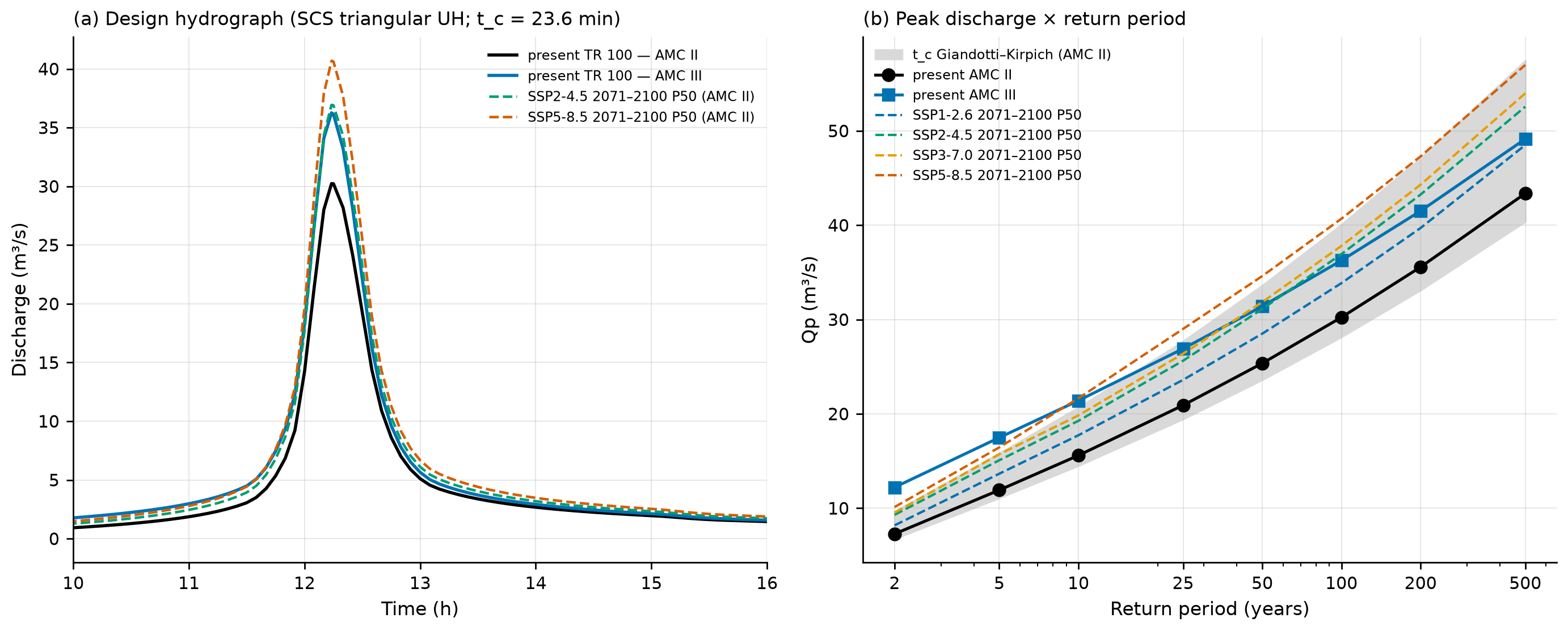
SCS triangular unit hydrograph. \(t_{lag} = 0.6\,t_c\); \(t_p = \Delta t/2 + t_{lag}\); \(t_b = 2.67\,t_p\); \(q_p = 0.208\,A\,P_e/t_p\) (NRCS NEH-630, ch. 16). To discretize the UH well (Δt ≤ 0.25·t_p), the 24-h rainfall was arranged in 5-min alternating blocks — the shortest duration of the DAEE/CETESB cascade — and subdivided into 1-min steps for the convolution (t_p = 14.6 min). The mass balance closes with zero error.

Table 8.13: Effective rainfall and peak discharge of the design hydrograph (present; chuva/hidrograma_resumo.json). The peak occurs at 734–736 min (12 h 14 min to 12 h 16 min).

TR	P24h (mm)	imax 5 min (mm/h)	Pe AMC II (mm)	C	Qp AMC II (m³/s)	Qp AMC III (m³/s)	Qp Kirpich / Giandotti (AMC II)
2	108.6	137.8	43.2	0.40	7.28	12.22	9.6 / 6.8
5	142.5	180.7	69.4	0.49	11.92	17.48	15.8 / 11.1
10	167.7	212.6	90.3	0.54	15.59	21.41	20.7 / 14.5
25	203.0	257.5	120.9	0.60	20.91	26.91	27.7 / 19.5
50	232.1	294.4	146.9	0.63	25.36	31.41	33.6 / 23.6
100	263.7	334.3	175.7	0.67	30.23	36.26	40.1 / 28.2
200	297.9	377.8	207.5	0.70	35.57	41.51	47.1 / 33.1
500	347.9	441.2	254.6	0.73	43.37	49.14	57.4 / 40.4

As a check, the rational method of Annex 1 of the manual, Q = C·I·A/3.6 with I(t_c) from Equation 8.1 and C from 0.75 to 0.95 (mountainous terrain, TR 100), gives 29.6–37.5 m³/s for TR 100 — the same range as the SCS hydrograph with AMC II and III.

Figure 8.19: Design hydrograph. (a) TR 100: present with AMC II and III, and end of century (P50, SSP2-4.5 and SSP5-8.5). (b) Peak discharge by TR, with the t_c range (Giandotti–Kirpich) and the climate scenarios.

scripts/casos/petropolis/03_cn_hidrograma.py (excerpt)

from trigrs_mapper.hydro import hidrograma as HD, scs_cn as SC

cn2 = 72.62                                   # BHAE 2022, cn2.ana_med (DPM database)
cn3 = SC.cn_condicao_umidade(cn2, "III")      # 85.9
pr = HD.hidrograma_projeto(h1min, area_km2=0.7712, cn=cn2, tc_hours=23.55 / 60)
print(pr.resumo()["qp_m3s"])                  # 30.2 m³/s for TR 100

The debris-flow peak discharge (Qsp) uses these Qp values and is computed in Section 8.7.6.

8.5.7 Rainfall of the February 15 and March 20, 2022 events

For the calibration (Section 8.9) we need the event hyetograph. Because the Cemaden hourly series is not accessible (the download requires a CAPTCHA) and MERGE does not capture the convective cell, the hyetograph was constructed from the published values and a documented temporal pattern (decision D14):

1. 3-h core (16:20–19:20, discretized as 16–19 h): 252.8 mm at São Sebastião, with the peak of 103.4 mm/h in the 2nd block; the 1st and 3rd blocks share the remainder in the proportion of MERGE in the same hours (79.8 and 69.6 mm).
2. 24-h total = 260 mm: the remaining 7.2 mm go to the following two hours, with the MERGE pattern.
3. Scaling to the watershed, 2–2.5 km east of the core stations: central scenario = INEA Alto da Serra (223 mm), in the same Palatinado River system; maximum = São Sebastião (260 mm); minimum = Bingen (142 mm), representative of the outer ring (131–147 mm).
4. Antecedent rainfall: 30 days of daily rainfall from ANA station 02243010 Itamarati-SE (DPM database; the observer records the rain on the day it falls).

Table 8.14: Constructed hyetograph of February 15, 2022 (mm per hour; chuva/evento_meta.json).

Local time (Feb 15)	16–17	17–18	18–19	19–20	20–21	24-h total	Peak (mm/h)
Minimum (Bingen)	43.6	56.5	38.0	2.0	1.9	142	56.5
Central (INEA Alto da Serra)	68.5	88.7	59.7	3.1	3.1	223	88.7
Maximum (São Sebastião)	79.8	103.4	69.6	3.6	3.6	260	103.4

Antecedent condition. At Itamarati-SE it rained 19.0 mm in 5 days, 85.6 mm in 10 days, 162.6 mm in 21 days, and 177.6 mm in 30 days before February 15 (Xavier: 267.4 mm in 30 days). This is much less than the 350 mm in 21 days published for Cemaden stations — a factor of 2.15 — further evidence of the spatial gradient. In TRIGRS, this uncertainty is not a factor of the sensitivity analysis: the antecedent rainfall enters through the background infiltration, which the calibration samples over a range (Section 8.9). The suggested background infiltration for TRIGRS is rizero = max(P30 − ETo30, 0)/30 d = (177.6 − 119.0) mm/30 d = 2.3×10⁻⁸ m/s, within the range of the parameter table (10⁻⁹ to 5×10⁻⁸ m/s; chuva/antecedente.json).

March 20, 2022 (planned validation, not yet run in TRIGRS). Hyetograph constructed with: 217.4 mm in 4 h (14–18 h), a peak block of 100 mm/h (Cemaden: “> 100 mm in 1 h”), and the remainder by the DAEE/CETESB increments; 415 mm in 10 h (until 24 h); and the early-morning pulse of March 21 with the MERGE pattern up to a total of 548 mm/24 h (Ochi et al., 2022). The minimum and central scenarios inherit the spatial ratios of February 15 (142/260 and 223/260; an assumption): 299, 470, and 548 mm. The three weeks before March 20 were almost dry (2 mm in 21 days at Itamarati-SE), and the suggested rizero falls to the floor of 10⁻⁹ m/s (chuva/evento2_*.json). The files evento_hietograma.csv and evento2_hietograma.csv give the time relative to the start of the window, with the antecedent period in daily steps and the event in hourly steps.

Figure 8.20: Rainfall of the 2022 events. (a, c) Daily antecedent rainfall (Itamarati-SE; in c, February 15 with the central total of event 1). (b, d) Constructed hyetographs: central (bars), maximum and minimum (steps). Hours > 24 belong to the following day.

WarningThe central limitation of this case

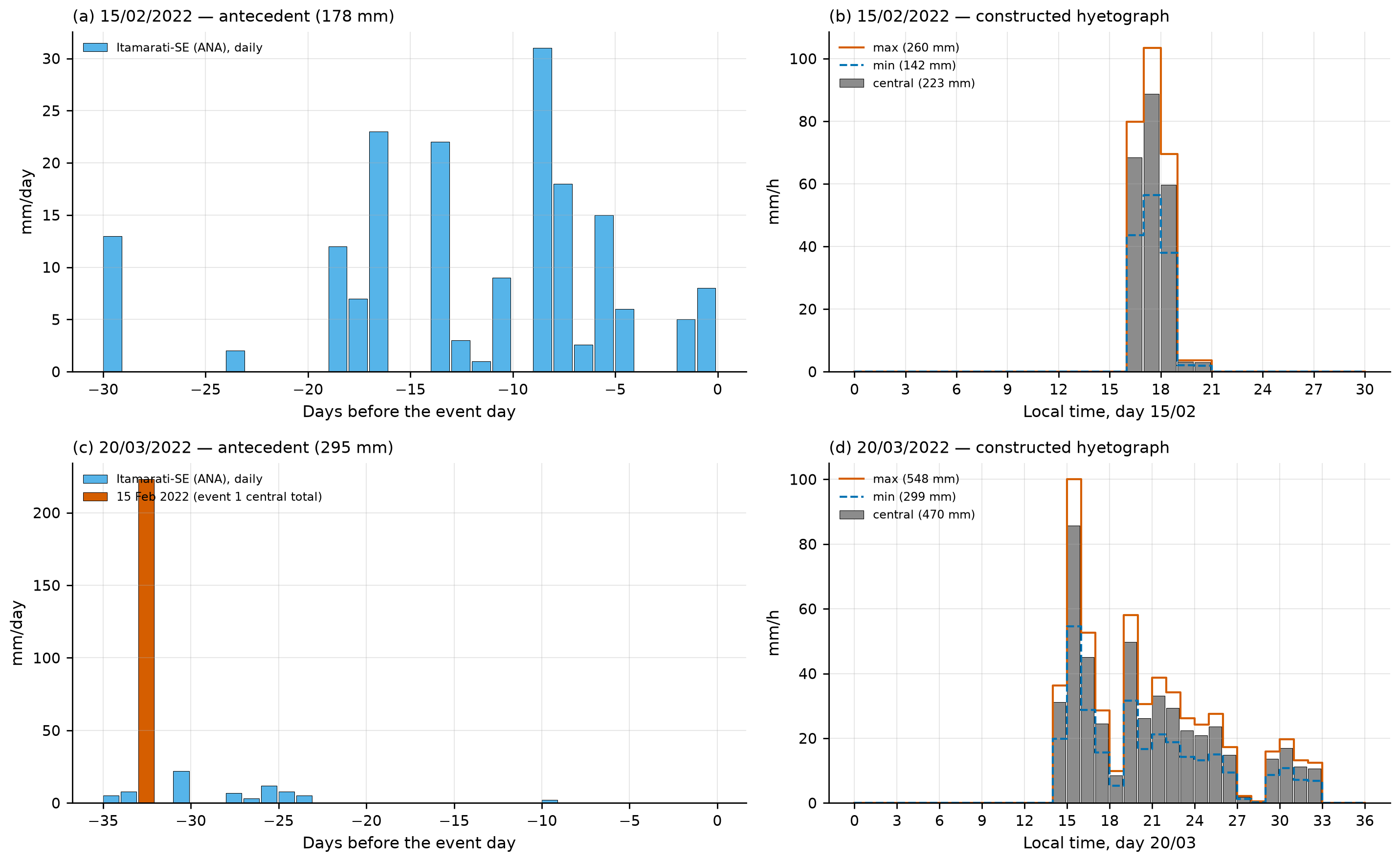
The hourly pattern of the events is constructed, not observed, and the rainfall over the watershed is unknown (the Cemaden rain gauge at Morin appears without data in Fig. 5a of Alcântara et al., 2023). Before the final calibration, the hourly series of Cemaden (São Sebastião, Dr. Thouzet, Morin) and INEA (Alto da Serra) should be obtained.

8.6 Climate change

The method is that of the IDF-MC Portal (SEDEC/MIDR; data version 2026.08.002), validated against the portal’s public API with a maximum relative difference of 1.6×10⁻⁷ (docs/pesquisa/07_mudanca_climatica.md). For each NEX-GDDP-CMIP6 model (0.25°; Thrasher et al., 2022), a Gumbel distribution is fitted by moments to the annual 1-day maxima in the model’s own historical run (1950–2014) and in the future window; the change factor FC is the ratio of the quantiles with the same TR:

\[ FC_m(T) = \frac{x_{T,\text{future}}}{x_{T,\text{historical}}},\qquad Pd_{\text{fut}}(T) = FC(T)\cdot Pd_{\text{obs}}(T) \tag{8.3}\]

and the model ensemble is summarized by P10, P50, and P90 — spread among models, not a confidence interval. The reference point falls in cell 2690547 (the main Petrópolis point in IDF-MC), 3.2 km from the cell’s northern edge — the same cell used in report 07. Since the disaggregation ratios are constant, the future IDF curves and hyetographs are those of the present multiplied by the FC of the corresponding TR (Figure 8.18).

Figure 8.21: Change factors FC(TR) for 2041–2070 and 2071–2100: P50 with P10–P90 bars for the four SSPs (n = number of models).

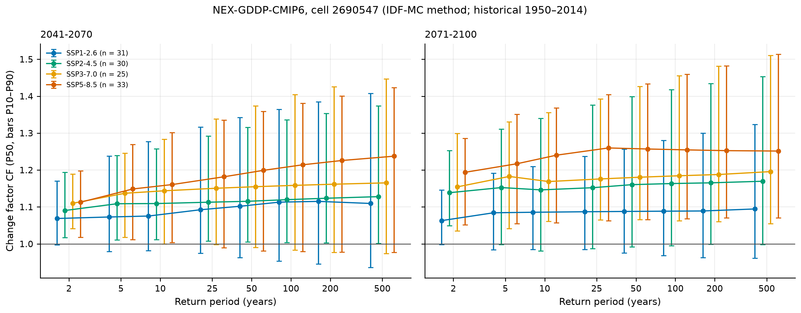
Table 8.15: Change factors and future TR 100 design rainfall (chuva/clima.json, chuva/pd_futuro.csv).

Scenario	2041–2070: FC P50 [P10–P90]	Pd100 (mm)	2071–2100: FC P50 [P10–P90]	Pd100 (mm)	Models with FC > 1 (end of century)
Present	—	233.3	—	233.3	—
SSP1-2.6 (31 models)	1.113 [0.954–1.365]	259.7 [222.5–318.4]	1.089 [0.968–1.280]	254.0 [225.9–298.6]	81%
SSP2-4.5 (30)	1.120 [1.004–1.336]	261.3 [234.2–311.7]	1.163 [0.995–1.417]	271.4 [232.2–330.7]	87%
SSP3-7.0 (25)	1.158 [0.983–1.405]	270.3 [229.4–327.7]	1.185 [1.063–1.455]	276.4 [248.0–339.6]	96%
SSP5-8.5 (33)	1.214 [0.979–1.381]	283.3 [228.5–322.2]	1.255 [1.068–1.459]	292.7 [249.2–340.5]	97%

For TR 200, the P50 goes from 263.7 mm (present) to 307.2 mm (SSP2-4.5, end of century) and 330.2 mm (SSP5-8.5, end of century). By the end of the century, the model median indicates an increase of 9% (SSP1-2.6) to 25% (SSP5-8.5) in the TR 100 daily rainfall, with an inter-model range as wide as the signal itself.

Equivalent TR. The question “how often will today’s TR 100 rainfall occur?” is answered by solving \(FC_m(T)\,x_{obs}(T) = x_{obs}(100)\) for each model, with the case’s GEV baseline, and summarizing P10/P50/P90 across models (Table 8.16, Figure 8.22).

Table 8.16: Future equivalent TR of today’s TR 100 rainfall (P10 = most severe; bounds [1.01; 10,000] years). The last column uses the IDF-MC method (scaling of α and β of the manual’s Gumbel) for comparison.

Scenario	2041–2070: P50 [P10–P90] (years)	2071–2100: P50 [P10–P90] (years)	IDF-MC method, Gumbel (P50, end of century)
SSP1-2.6	58.1 [23.6–133.2]	63.0 [31.4–121.2]	50.5
SSP2-4.5	54.9 [25.6–97.9]	45.2 [19.4–102.7]	33.1
SSP3-7.0	45.9 [22.2–111.3]	41.0 [18.7–71.7]	28.0
SSP5-8.5	38.7 [22.2–113.1]	29.2 [17.9–70.1]	20.8

Figure 8.22: (a) Present and future Pd(TR) (P50 of the four SSPs; SSP5-8.5 P10–P90 band at the end of the century). (b) Equivalent TR of today’s TR 100 rainfall.

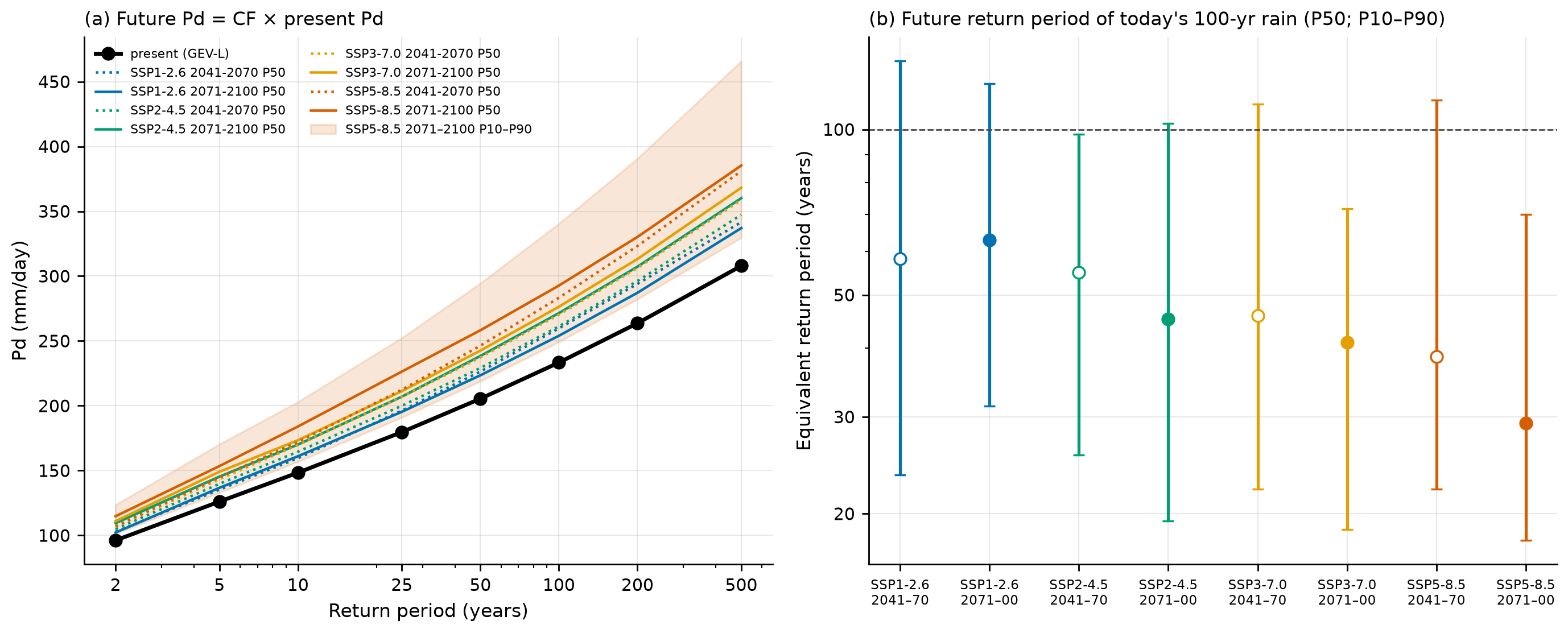
With the heavy tail of the GEV, the same relative increase in rainfall shifts the TR less than with the Gumbel: under SSP5-8.5, at the end of the century, today’s TR 100 rainfall acquires a median TR of 29 years by the GEV and 21 years by the IDF-MC method. Either way, today’s 100-year event becomes something like a 20- to 60-year event by the end of the century, depending on the scenario.

WarningLimitations of the climate factors

1. The cell covers ~700 km² and the watershed 0.77 km²; (ii) the Gumbel is imposed in both windows, and the FC for TR ≥ 100 is an extrapolation from the 30-year future window; (iii) daily rainfall only — the increase in sub-daily rainfall and in multi-day antecedent rainfall is not represented; (iv) no probabilities are assigned to the SSPs.

8.7 The traditional GIDES/JICA method

We follow chapter 2 of the technical manual on debris flows (Brasil/MI-SEDEC and JICA, 2018/2019) with the trigrs_mapper.sabo module, which exactly reproduces Appendix A (Nova Friburgo). The watershed has 0.77 km² (< 5 km², the method’s limit of application). Script: scripts/casos/petropolis/05_gides.py; results in gides/gides.json and gides/tabelas/*.csv.

8.7.1 Parameters Kf2 and Cd

\[ K_{f2} = 0.05\,(\log_{10}A - 2)^2 + 0.05 = 0.05\,(\log_{10}0.7712 - 2)^2 + 0.05 = 0.273 \tag{8.4}\]

within the limits [0.1; 0.5]. Takahashi’s equilibrium concentration uses the mean slope over the 200 m upstream of the point (NILIM TN 904; minimum of 10°), θ = 18.0°, with σ = 2,600 kg/m³, ρ = 1,200 kg/m³, and φ = 35°:

\[ \begin{aligned} C_d &= \frac{\rho\tan\theta}{(\sigma-\rho)(\tan\phi-\tan\theta)} = \frac{1{,}200\times0.325}{1{,}400\times(0.700-0.325)} = 0.742\\[4pt] &\Rightarrow\ C_d = 0.9\,C^* = \mathbf{0.54} \end{aligned} \tag{8.5}\]

The cap of 0.54 is reached for θ ≥ ~15.1° (Table 8.17): with θ = 15.1° (local 50-m slope), C_d = 0.537; with θ = 10°, it would drop to the floor of 0.30. With ρ = 1,000 kg/m³ the result is also 0.54.

Table 8.17: Sensitivity of C_d, K_q, and V_dy2 to the slope θ (gides/tabelas/sensibilidade_theta_cd.csv).

θ (°)	10	12	14	15.1	16	18	20
Cd	0.300	0.374	0.474	0.537	0.540	0.540	0.540
Kq = C*/(C* − Cd)	2.0	2.65	4.76	9.58	10.0	10.0	10.0
Vdy2 TR 100 (m³)	35,115	48,870	73,830	95,170	96,184	96,184	96,184

8.7.2 Vdy11: channel-bed sediment (order ≥ 1)

\(V_{dy11} = \sum B_d\,D_e\,L_{dy11}\). Without a field survey, we adopt an erodible cross section of 20 m² (B_d = 10 m × D_e = 2 m), anchored on Appendix A: B_d = 10 m at the valley outlet and an equivalent erodible section of the surveyed thalweg of 10,873 m³ / ~500 m ≈ 22 m². The manual notes that, in Japan, D_e rarely exceeds 5 m in the channel. The DEM-based B_d (median of 28 m) is an upper bound, because it is below the resolution of ANADEM; the hydraulic width from BHAE-HGM (hydraulic-geometry attributes; 2.7 m, in a 10.5-km² unit) is that of the water channel, not of the erodible bed.

Table 8.18: Vdy11 by Strahler order (gides/tabelas/vdy1_metodo_b_trechos.csv).

Order	Ldy11 (m)	Ady11 (m²)	Vdy11 (m³)
1	3,553	20	71,066
2	816	20	16,320
3	514	20	10,272
4	886	20	17,728
Total	5,769	—	115,386

8.7.3 Traditional Vdy12: hillslope failures

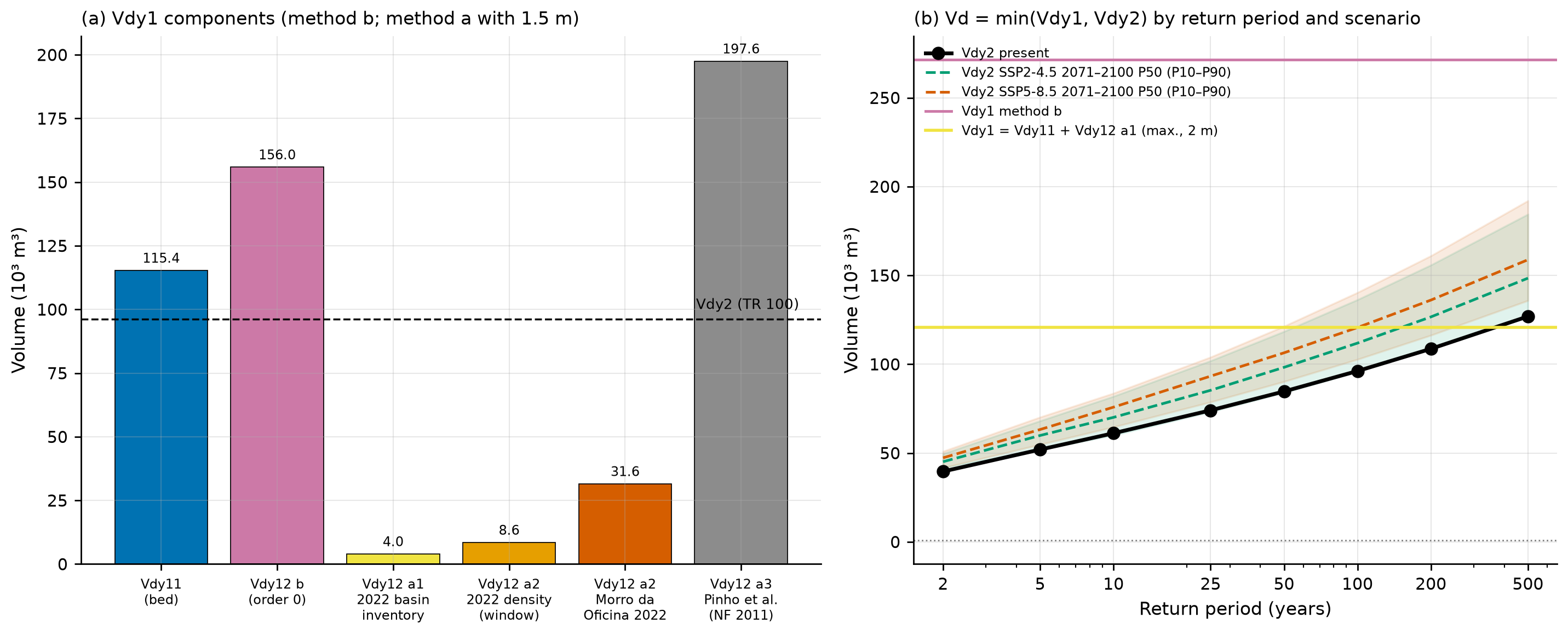
Method “b” (zero-order thalwegs). With the same logic (“analogously” to the bed, §2.5.1.1 b), B_d = 10 m and D_e = 1.5 m (shallow landslides of 0.5–2 m in the Serra do Mar): Ady12 = 15 m² and V_dy12 = 15 m² × 10,396.7 m ≈ 155,950 m³ (the Ldy12 of 10,397 m in Table 8.5, unrounded).

Method “a” (scars). The manual allows V_dy12 to be estimated from failure maps. We use scar area × a thickness of 1–2 m, in situ — without bulking, as the manual allows in preliminary studies (“this effect may be neglected”, §2.5.1.1 a), and on the same basis as V_dy11 (form (i) of project decision D18; the porosity-corrected and “loose” (bulked) forms will be used in the coupling with TRIGRS, Section 8.10) — in three variants (Table 8.19):

• a1 — 2022 inventory within the watershed: Sentinel-2 candidates of exposed soil. After February 15 (scene of March 4, 2022), the base rule found no scars in the watershed and the calibrated rule found 1,000 m²; including the March 20 event (scene of April 23, 2022), 2,700 m².
• a2 — 2022 density of Alto da Serra transferred to the watershed: scar area per area with slope ≥ 15°, applied to the 627,600 m² of the watershed with slope ≥ 15°. In the calibration window the density is 0.91% (193,400 m² of scars); in a 1-km disk at Morro da Oficina, 3.36%.
• a3 — density by slope class from Pinho et al. (2013), Córrego D’Antas in 2011 (Table 3.1 of Appendix A of the manual): 0.03 to 0.40 ha/ha depending on the class, equivalent to 17% of the watershed.

Table 8.19: V_dy12 by method “a” (m³, in situ — form (i) of decision D18, comparable to V_dy11; the upper bound V_solto (loose, bulked) = V_insitu/(1 − 0.4) multiplies by 1.67). Source: gides/tabelas/vdy12_metodo_a_variantes.csv.

Variant	Scar area (m²)	Vdy12 with 1 m	1.5 m	2 m
a1 — S2 Mar 4, 2022, base rule	0	0	0	0
a1 — S2 Mar 4, 2022, calibrated rule	1,000	1,000	1,500	2,000
a1 — S2 Apr 23, 2022, calibrated rule (Feb 15 + Mar 20)	2,700	2,700	4,050	5,400
a2 — density of the 2022 calibration window	5,703	5,703	8,554	11,406
a2 — Morro da Oficina 2022 density	21,061	21,061	31,591	42,122
a3 — Pinho et al. (2013), NF 2011	131,702	131,702	197,553	263,404

The comparison is instructive: method “b” (156 thousand m³) is equivalent to assuming that the whole watershed behaves like Córrego D’Antas in 2011, the most severe case in the Rio de Janeiro Highlands; in 2022, with rainfall comparable to a TR of 40–90 years, the Morin watershed had practically no detectable failures. This is the gap that TRIGRS must fill: estimating how much of the hillslopes fails under each rainfall (Section 8.10).

8.7.4 Vdy1, Vdy2, and the design volume Vd

\[ \begin{aligned} V_{dy1} &= V_{dy11} + V_{dy12}\\[4pt] V_{dy2} &= \frac{10^3\,P_p\,A}{1-K_v}\cdot\frac{C_d}{1-C_d}\cdot K_{f2}\\[4pt] V_d &= \max\left[\min(V_{dy1}, V_{dy2}),\ 1{,}000\ \text{m}^3\right] \end{aligned} \tag{8.6}\]

with K_v = 0.4 and P_p = 1-day Pd(TR) (as in Appendix A, which used 191 mm = daily P200). By method “b”, V_dy1 = 115,386 + 155,950 = 271,336 m³. For TR 100 (the manual’s minimum for Sabo dams):

\[ V_{dy2} = \frac{10^3\times233.33\times0.7712}{0.6}\times\frac{0.54}{0.46}\times0.2732 = \mathbf{96{,}184\ m^3} \]

The calculation uses unrounded P_p and K_f2 (233.33 mm and 0.2732); with 233.3 mm and 0.273, it would give 96,101 m³.

Table 8.20: Design volumes in the present climate (gides/gides.json).

TR (years)	2	5	10	25	50	100	200	500
Pp (mm)	96.1	126.1	148.4	179.7	205.4	233.3	263.7	307.9
Vdy2 (m³)	39,635	51,975	61,160	74,069	84,684	96,184	108,686	126,932
Vd (sediment), method b	39,635	51,975	61,160	74,069	84,684	96,184	108,686	126,932
Governing term	Vdy2	Vdy2	Vdy2	Vdy2	Vdy2	Vdy2	Vdy2	Vdy2
Vd with Vdy12 “a1” (2 m)	39,635	51,975	61,160	74,069	84,684	96,184	108,686	120,786 (Vdy1)

In Petrópolis, V_dy2 governs: the volume is limited by the transport capacity of the rainfall, not by sediment availability — the opposite of Appendix A in Nova Friburgo (V_dy1 = 10,873 < V_dy2 = 22,422 m³). The consequence for climate change is direct: since V_dy2 is linear in P_p, the design volume grows in the same proportion as the rainfall (Table 8.21). With V_dy12 from the 2022 inventory (variant a1), however, V_dy1 drops to 120,786 m³ and becomes the governing term at TR 500 and in the most severe future scenarios — which term governs depends on how much of the hillslopes fails, precisely the question TRIGRS addresses.

Table 8.21: V_dy2 under climate change (end of century). All scenarios and horizons in gides/tabelas/vdy2_vd_qsp_tr_cenarios.csv.

Scenario (2071–2100)	Vdy2 TR 100 (m³), P50 [P10–P90]	Vdy2 TR 200 (m³), P50
Present	96,184	108,686
SSP2-4.5	111,898 [95,733–136,334]	126,656
SSP5-8.5	120,666 [102,728–140,369]	136,126

8.7.5 Woody debris (Vwy)

\(V_{wy} = (B_d\,L_{dy13}/100)\,\Sigma V_{wy2}\) with \(V_{wy2} = (\pi\,DAP^2/4)\,H_w\,K_d\). We use the density (8 trees/100 m²), the DAP (diameter at breast height, DBH; 0.25 m), and the K_d (0.6) of Appendix A — surveyed in the same forest type (Montane Dense Ombrophilous Forest) — and the height H_w = 17 m, the median canopy height from GLAD 2010 in the watershed, instead of the 6 m of Appendix A. With B_d = 10 m and L_dy13 = 2,177 m (main thalweg, from the point to the divide): V_wy2 = 0.50 m³, ΣV_wy2 = 4.01 m³/100 m², V_wy = 872 m³ and, with K_w = 0.9 (manual, no countermeasures), V_w = 785 m³. With the Appendix A parameters (H_w = 6 m), V_wy = 308 m³; with the whole network of order ≥ 1 (5,769 m), 2,311 m³ (gides/tabelas/vwy_troncos.csv). Woody debris accounts for less than 1% of the total volume.

Total plan volume (TR 100): 96,184 + 785 = 96,969 m³, or about 126 thousand m³/km².

8.7.6 Debris-flow peak discharge (Qsp)

The manual (Annex 1) calls for the calculation by two paths and the adoption of the larger value:

• Empirical: \(Q_{sp} = 0.002\,\Sigma Q\), \(\Sigma Q = C^*\,V_{dqp}/C_d\). The Japanese standard from which the relation comes (NILIM TN 904, Eq. 10) uses 0.01, five times more; we report both.
• Rational: \(Q_{sp} = K_q\,Q_p\), \(K_q = C^*/(C^* - C_d) = 0.6/(0.6-0.54) = 10.0\), with Q_p from the design hydrograph (Table 8.13).

Table 8.22: Debris-flow peak discharge (m³/s) in the present climate (gides/gides.json).

TR	ΣQ (m³)	Qsp = 0.002·ΣQ	Qsp = 0.01·ΣQ	Kq·Qp AMC II	Kq·Qp AMC III	Adopted (larger of 0.002·ΣQ and Kq·Qp II)
10	67,956	135.9	679.6	155.9	214.1	155.9
50	94,093	188.2	940.9	253.6	314.1	253.6
100	106,872	213.7	1,068.7	302.3	362.6	302.3
200	120,762	241.5	1,207.6	355.7	415.1	355.7

ImportantA clue about the coefficient: 0.002 vs. 0.01

Annex 1 states that, with a specific volume of ~100,000 m³/km², a 24-h rainfall of 260 mm, and a watershed smaller than 1 km², the rational method should give a smaller value than the empirical one. Petrópolis is exactly under these conditions (126 thousand m³/km², 264 mm in 24 h for TR 100, 0.77 km²). Here, K_q·Q_p = 302 m³/s is larger than 0.002·ΣQ = 214 m³/s and smaller than 0.01·ΣQ = 1,069 m³/s: only the Japanese coefficient is consistent with the manual’s own statement. The discrepancy is recorded, to be resolved with the SABO Project team.

8.7.7 Sensitivity and comparison with analogous watersheds

• Erodible cross section (B_d, D_e) — with B_d from 2.7 to 28 m and D_e from 1 to 5 m, V_dy1 by method “b” ranges from 43.6 thousand to 2.26 million m³ (gides/tabelas/sensibilidade_bd_de.csv). With method “b”, V_dy2 governs at TR 100 whenever B_d·D_e > 6.0 m²; considering only the bed (V_dy11), whenever B_d·D_e > 16.7 m².
• Channel threshold — V_dy1 “b” ranges from 162.7 thousand m³ (5 ha) to 687.6 thousand m³ (0.25 ha); with the 30-m DEM, 311.6 thousand m³.
• Area (10 vs. 30 m) — 0.7712 and 0.7785 km² change V_dy2 TR 100 by 0.6% (96,184 vs. 96,788 m³).
• Slope θ — Table 8.17: C_d and K_q only drop if θ < 15°.

Table 8.23: Comparison with the manual’s case and with volumes observed in 2022. There is no official Sabo design for this watershed. Sources: GIDES manual, Appendix A; Custódio et al. (2023); Ochi et al. (2022).

Case	A (km²)	Pp (mm; TR)	Vdy1 (m³)	Vdy2 (m³)	Plan volume (m³)	m³/km²	Governs
Nova Friburgo — Appendix A of the manual	0.12	191 (200)	10,873	22,422	10,928	91,067	Vdy1
Petrópolis — this chapter	0.77	233.3 (100)	271,336	96,184	96,969	125,738	Vdy2
Morro da Oficina, Feb 15, 2022 (single scar)	—	260 (event)	—	—	15,763–31,526 (1–2 m)	—	—
2022 municipal inventory (mean per failure)	—	—	—	—	1,600–3,200 (1–2 m)	—	—

The Petrópolis design volume is equivalent to three to six times the largest 2022 scar (Morro da Oficina) or to 30–60 average failures of the municipal inventory concentrated in a single 0.77-km² watershed — a conservative envelope, as expected from the method.

Figure 8.23: GIDES method. (a) Components of V_dy1: bed, zero order (method b), and the method-a variants with a 1.5-m thickness, compared with V_dy2 TR 100. (b) V_dy2 by TR in the present and at the end of the century (P50 and P10–P90), and V_dy1 by methods b and a1.

scripts/casos/petropolis/05_gides.py (excerpt)

from trigrs_mapper import sabo as S

kf2 = S.kf2(0.7712)                            # 0.273
cd = S.cd_takahashi(18.0).cd                   # 0.742 -> 0.54 (cap 0.9·C*)
v2 = S.vdy2_m3(233.328, 0.7712, cd, kf2)       # 96,184 m³ (TR 100; unrounded Pp)
vd = S.volume_projeto(271_336, v2, vw=785)     # governs: Vdy2; total 96,969 m³
qsp = S.qsp_envelope(S.soma_q_m3(vd["volume_sedimentos_m3"], cd))
print(vd, qsp, S.kq(cd) * 30.23)               # Kq·Qp = 302 m³/s

8.8 TRIGRS modeling

Sections 8.1 to 8.7 prepared everything TRIGRS needs: the DEM and the drainage network, the soil, geology, and land-cover datasets, the design rainfall (present and future), and the hyetograph of the February 15, 2022 storm. This section shows how these layers become the input files of TRIGRS 2.1 (Baum, Savage & Godt, 2008; Baum, Godt & Savage, 2010) and which runs were made. The theory of the model is in chapter 1, and the setup is explained in more detail in the Nova Friburgo chapter; here we keep the choices and numbers of Petrópolis.

NoteWhere the TRIGRS numbers come from

The TRIGRS results come from the project pipeline (trigrs_mapper package, command trigrs-mapper caso petropolis <step>; Section 8.12) and enter the text through a generator (scripts/capitulos/gerar_resultados_trigrs.py) that reads the files in data/cases/petropolis/ and writes the tables and the values quoted: no TRIGRS result was typed by hand. The values in this version come from the full run (decisions D20 and D21; state of the results: final). If the pipeline is run again, it is enough to run the generator once more: tables, values, and figures change together, and a warning appears at the start of this section if any source stops coming from the full run or no longer agrees with the case configuration. An “n/a” would mark a value that the run did not produce.

8.8.1 Computational domains

TRIGRS runs on three domains (Table 8.24), each with its own grids and NODATA mask — the program requires NODATA in the same cells in all input grids.

Table 8.24: Domains of the Petrópolis TRIGRS runs.

Domain	Purpose	Resolution	Size
Morin watershed (reference point of Section 8.2)	event in the watershed, design runs (TR × climate), thresholds, and Forecast tab	10 m (30 m for the thresholds; 30 m in the resolution comparison)	0.771 km²; 7,712 10-m cells
Alto da Serra/Morro da Oficina window (PET_calibracao_2022)	calibration, sensitivity, and event metrics	30 m	31,185 valid cells (28.1 km²)
Vale do Cuiabá window (PET_CUI_calibracao_2011)	cross-validation with the 2011 inventory and the Teresópolis rainfall (overlapping the Teresópolis area: not independent)	30 m	— (outside the case’s 12-km window; ANADEM reprojected with a 2-km margin)

The calibration is done at 30 m, the native resolution of ANADEM, because a 10-m run costs about nine times more and the search requires hundreds of runs (decision D12). The calibrated multipliers are then applied to the 10-m watershed — bicubic resampling creates no information (D5), and the sensitivity to resolution is reported in Section 8.9.

The grades (grids) step generates, in each domain: the conditioned DEM (the same as in Section 8.4, used by TopoIndex), the slope (Horn, 1981, computed on the raw DEM), the D8 directions in the TopoIndex scheme, the contributing area, the channel (A ≥ 1 ha, the threshold of Section 8.4), the plan and profile curvatures (Zevenbergen & Thorne, 1987), and the topographic wetness index. Slope, curvatures, and contributing area feed the unit and thickness rules below.

8.8.2 Geotechnical units and property zones

Each cell receives a geotechnical unit from the first rule it satisfies, in the order of Table 8.25 (project report 04, docs/pesquisa/04_parametros_trigrs.md):

Table 8.25: Rules of the geotechnical units (trigrs_mapper.params); “—” = only the general 5-m cap.

Priority	Unit	Rule	zmax cap
1	rock outcrop	MapBiomas class 29 (outcrop) in 2015	0.1 m
2	talus/alluvial deposit	Quaternary geology (Q*) or valley floor: A ≥ 1 ha and β < 10°	—
3	colluvium	concavity (plan curvature < 0) with A ≥ 0.25 ha (zero-order thalwegs)	—
4	shallow soil over rock	neighborhood of the outcrop (8 cells) or IBGE soil unit whose dominant component is AR (rock outcrops)	0.5 m (neighborhood); 1.0 m (AR unit)
5	mature residual soil	remaining hillslopes, split by the 1:100,000 lithology (granite × orthogneiss)	—

In Petrópolis, two rules matter. First, the 1:250,000 IBGE soil map used by the pipeline places 86% of the watershed — its entire upstream part — in unit AR3 (rock outcrops associated with Cambisols and Litholic Neosols) and only the downstream reach in CXbd32 (Section 8.3, Figure 8.6): this is why shallow soil over rock, with zmax ≤ 1 m, is the dominant unit (Table 8.26). Second, the whole watershed lies on the orthogneiss of the Rio Negro Complex (Figure 8.8), so the mature residual soil has a single lithology. The persistent MapBiomas outcrop is a small patch (Section 8.3).

Each unit is combined with a land-cover group, which sets the root cohesion C_r: forest (G1) 2 kPa and herbaceous vegetation, pasture, and mosaic (G3) 0.5 kPa as central values (José, 2016; report 04, §5). In the calibration and in the event run, the land cover is the one before the event (MapBiomas 2015 — the 2021 map could not be obtained and the 2025 map postdates the disaster); in the design runs and in the thresholds, the current one (MapBiomas 2025); in the Vale do Cuiabá validation, GLAD 2010. Each unit × lithology × group combination present in the domain becomes a zone of tr_in.txt, numbered 1 to N, with the properties

\[ \begin{aligned} c &= c'_0\,m_c + C_r\,m_{Cr}, & \tan\varphi' &= m_{\tan\varphi}\tan\varphi'_0,\\ K_s &= K_{s0}\,m_{K_s}, & D_0 &= r_{D_0}\,K_s,\\ \alpha &= \alpha_0\,m_\alpha, & \gamma_s &= \gamma_w\left[G_s\,(1-\theta_s)+\theta_s\right] \end{aligned} \tag{8.7}\]

where the subscript 0 marks the central a priori values of report 04 (there are no laboratory tests in Petrópolis) and the m are the calibration multipliers (Section 8.9); θ_s, θ_r, and G_s stay at their central values. The outcrop is a conventional zone, very strong and practically impervious (c = 100 kPa, K_s = 10⁻⁹ m/s, α < 0), which the multipliers do not change. Because the land covers differ, the zone numbering changes from one run to another: Table 8.26 gives the design zones, the same as in the annotated tr_in.txt below, and Table 8.27, those of the event run in the watershed.

Table 8.26: TRIGRS property zones in the watershed — parameterization of the design runs (10 m; design land cover MapBiomas 2025: G1 forest; G3 grassland/pasture; 7 zones, numbered as in the annotated tr_in.txt) with the calibrated multipliers (full calibration, sample lhs_0014: m_c = 0.78, m_tanφ = 1.12, m_Ks = 4.22, r_D0 = 46 m, m_α = 0.60, m_Cr = 0.74). c′ = c′₀·m_c and c_r = C_r·m_Cr (total cohesion c = c′ + c_r); tan φ′ = m_tanφ·tan φ′₀; K_s = K_s0·m_Ks; D₀ = r_D0·K_s; α = α₀·m_α; γ_s derived from θ_s and G_s. The rock outcrop is the conventional, uncalibrated zone (α < 0: saturated infiltration). The event run uses the event land cover and a different numbering (event zone table).

Zone · unit (lithology) · land cover	c′ + cr (kPa)	φ′ (°)	γs (kN/m³)	Ks (m/s)	D0 (m²/s)	θs / θr	α (1/m)	Area (%)
1 · colluvium · G1	2.34 + 1.47	37.2	18.02	4.22 × 10⁻⁵	1.96 × 10⁻³	0.48 / 0.08	3.02	13.8
2 · colluvium · G3	2.34 + 0.37	37.2	18.02	4.22 × 10⁻⁵	1.96 × 10⁻³	0.48 / 0.08	3.02	< 0.1
3 · mature residual soil (orthogneiss) · G1	3.90 + 1.47	38.2	17.81	4.22 × 10⁻⁵	1.96 × 10⁻³	0.50 / 0.10	4.22	12.5
4 · shallow soil over rock · G1	1.56 + 1.47	40.3	18.50	8.44 × 10⁻⁵	3.92 × 10⁻³	0.45 / 0.06	3.62	66.2
5 · shallow soil over rock · G3	1.56 + 0.37	40.3	18.50	8.44 × 10⁻⁵	3.92 × 10⁻³	0.45 / 0.06	3.62	4.6
6 · talus/alluvium deposit · G1	0.78 + 1.47	39.2	19.60	2.11 × 10⁻⁴	9.79 × 10⁻³	0.38 / 0.05	4.83	1.7
7 · rock outcrop	100.00 + 0.00	45.0	26.00	1.00 × 10⁻⁹	1.00 × 10⁻⁷	0.05 / 0.01	< 0 (sat.)	1.2

Figure 8.24: TRIGRS property zones in the 10-m watershed (geotechnical unit × lithology × MapBiomas 2025 land cover). The colluvia trace the zero-order thalwegs; the shallow soil over rock covers the part of the watershed mapped as rock outcrops (AR3) on the 1:250,000 soil map; the residual soil of the orthogneiss lies in the downstream reach, next to the reference point.

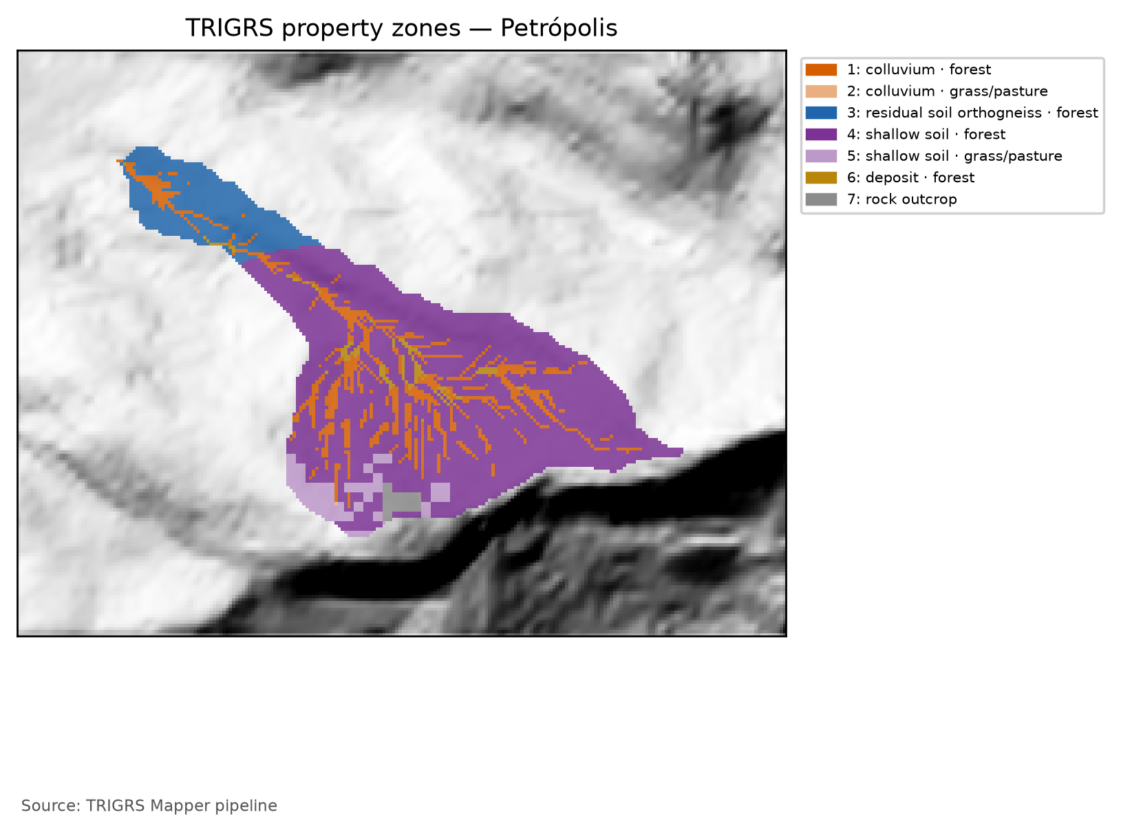
Table 8.27: TRIGRS property zones in the watershed — parameterization of the event run (10 m; event land cover MapBiomas 2015: G1 forest; G3 grassland/pasture; 6 zones, numbered independently of the design tr_in.txt) with the multipliers in use (full calibration, sample lhs_0014: m_c = 0.78, m_tanφ = 1.12, m_Ks = 4.22, r_D0 = 46 m, m_α = 0.60, m_Cr = 0.74). c′ = c′₀·m_c and c_r = C_r·m_Cr (total cohesion c = c′ + c_r); tan φ′ = m_tanφ·tan φ′₀; K_s = K_s0·m_Ks; D₀ = r_D0·K_s; α = α₀·m_α; γ_s derived from θ_s and G_s. The rock outcrop is the conventional, uncalibrated zone (α < 0: saturated infiltration). The calibration window (30 m) uses the same event land cover.

Zone · unit (lithology) · land cover	c′ + cr (kPa)	φ′ (°)	γs (kN/m³)	Ks (m/s)	D0 (m²/s)	θs / θr	α (1/m)	Area (%)
1 · colluvium · G1	2.34 + 1.47	37.2	18.02	4.22 × 10⁻⁵	1.96 × 10⁻³	0.48 / 0.08	3.02	13.8
2 · mature residual soil (orthogneiss) · G1	3.90 + 1.47	38.2	17.81	4.22 × 10⁻⁵	1.96 × 10⁻³	0.50 / 0.10	4.22	12.5
3 · shallow soil over rock · G1	1.56 + 1.47	40.3	18.50	8.44 × 10⁻⁵	3.92 × 10⁻³	0.45 / 0.06	3.62	69.1
4 · shallow soil over rock · G3	1.56 + 0.37	40.3	18.50	8.44 × 10⁻⁵	3.92 × 10⁻³	0.45 / 0.06	3.62	1.7
5 · talus/alluvium deposit · G1	0.78 + 1.47	39.2	19.60	2.11 × 10⁻⁴	9.79 × 10⁻³	0.38 / 0.05	4.83	1.7
6 · rock outcrop	100.00 + 0.00	45.0	26.00	1.00 × 10⁻⁹	1.00 × 10⁻⁷	0.05 / 0.01	< 0 (sat.)	1.2

Between 2015 and 2025, part of the forest became a mosaic of uses (from 1.7% to 4.8% of the watershed; chuva/cn.json): those cells move from group G1 to G3 and lose root cohesion, which affects the initial condition of the design runs (Section 8.10).

8.8.3 Unsaturated infiltration: the Gardner model

The pipeline uses the unsaturated model with a finite-depth base of TRIGRS 2.1 (Baum, Godt & Savage, 2010), recommended by report 04 because the mechanisms described in the Serra do Mar — loss of suction as the wetting front advances and a perched water table over the less permeable contact — depend on storage in the unsaturated zone. The retention curve and the conductivity follow the exponential model of Gardner (1958):

\[ \theta(\psi) = \theta_r + (\theta_s-\theta_r)\,e^{\alpha\psi},\qquad K(\psi) = K_s\,e^{\alpha\psi}\qquad (\psi \le 0) \tag{8.8}\]

The parameter α (1/m) tells how fast the soil loses water and conductivity with suction: a high α describes a coarse soil that drains easily; a low α, a fine soil, with a capillary fringe about 1/α high. In the factor-of-safety equation, the pressure head is weighted by the effective saturation χ, as in Baum, Godt & Savage (2010) (TRIGRS routine pstpf.f95):

\[ FS(Z,t) = \frac{\tan\varphi'}{\tan\delta} + \frac{c - \chi(Z,t)\,\psi(Z,t)\,\gamma_w\tan\varphi'}{\gamma_s\,Z\,\sin\delta\cos\delta}, \qquad \chi = \frac{\theta(Z,t)-\theta_r}{\theta_s-\theta_r} \tag{8.9}\]

Above the water table (ψ < 0), suction adds strength in proportion to saturation; below it, χ = 1 and the equation is the one in chapter 1, with c = c′ + c_r. In the zones with α > 0, tr_in.txt sets the unsaturated model for all cells, even where the initial capillary fringe reaches the surface; the outcrop (α < 0) uses saturated infiltration.

8.8.4 Soil thickness (zmax) and the bedrock cap

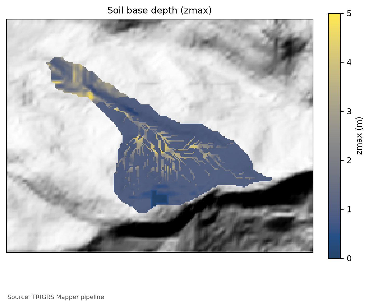
zmax is the low-permeability base of the model — the soil–rock or colluvium–saprolite contact where shallow failures form, at 1–2.5 m in the Serra do Mar (report 04, §6) — and not the depth to fresh rock. Without thickness measurements, the pipeline uses an exponential model of the slope β (in degrees) with caps by unit:

\[ z_{max} = \min\left\{T_u;\ \min\left[5;\ \max\left(0.3;\ 5.66\,m_z\,e^{-k_z\,\beta}\right)\right]\right\}\quad\text{(m)} \tag{8.10}\]

A priori, m_z = 1 and k_z = 0.0347/degree: the curve passes through 2.0 m at 30° and 1.0 m at 50°, close to those of DeRose (1996) and Salciarini et al. (2006); T_u is the cap of the unit (Table 8.25). The bedrock enters through these caps — 0.1 m on the outcrop, 0.5 m in its neighborhood, and 1.0 m in the AR unit of the soil map. BDTICM (7.9–14.1 m in the watershed; Figure 8.11) measures regolith and saprolite and always lies above the general 5-m cap: it does not limit zmax, and its spatial pattern only appears as an alternative model (“regolith”) in the sensitivity analysis. The calibration adjusts m_z and k_z (calibrated: 0.88 and 0.0410/degree; Table 8.30). Since thickness derived from slope alone was the worst option in the comparison by Segoni, Rossi & Catani (2012), the sensitivity analysis always tests alternative models.

Figure 8.25: Soil thickness zmax (m) in the 10-m watershed. Over most of the watershed, the 1.0-m cap of the AR unit prevails (shallow soil over rock); in the colluvia of the thalwegs and in the residual soil of the downstream reach, the slope model reaches several meters; the outcrop is set to 0.1 m.

8.8.5 Initial water table, background infiltration, and the initial condition

There are no water-table measurements in Petrópolis. The initial condition is a water table at a depth depthwt in each cell, in two families:

• Working configuration: depthwt = f_NA·zmax, with f_NA ∈ {0.5; 0.75; 1} among the calibration parameters (f_NA = 1 is the water table at the base of the soil, the central value of report 04). Calibrated: f_NA = 0.50.
• Scenarios of decision D6: depthwt = min(d, zmax), with d = 1, 2, …, 10 m — the water table capped at the bedrock contact —, used in the sensitivity analysis and in the thresholds.

There is a practical consequence: where zmax ≤ 1 m — most of the watershed —, all scenarios with d ≥ 1 m put the water table at the base of the soil and are identical; they only differ in the colluvia, the residual soil, and the deposits, where the soil is thicker (Figure 8.26).

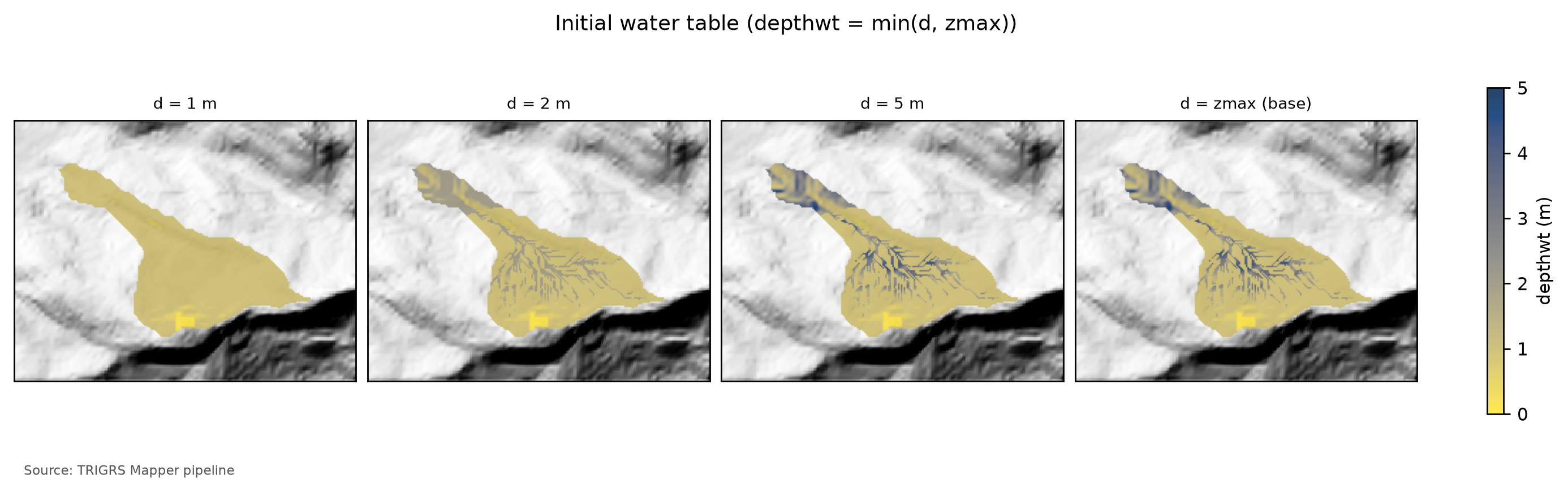
Figure 8.26: Initial water table depthwt = min(d, zmax) in the watershed for d = 1, 2, and 5 m and for the water table at the base of the soil (d = zmax). Where the soil is up to 1 m thick, the four panels coincide; the differences appear in the colluvial thalwegs and in the downstream reach.

f_NA is an effective parameter, not a measured water table. Without observations, f_NA condenses into a single initial condition the moisture left by the rains of the previous weeks: the smaller f_NA, the higher the water table — with 0.5, it fills the lower half of the soil, a wet, storm-like state. The volumes of the following sections hold for this initial condition, kept the same in the present and in the future; the D6 scenarios and the fractions 1, 0.75, and 0.5 of the sensitivity analysis (Section 8.9) show how much it matters.

The rainfall of the previous months enters as a steady background infiltration, rizero. The antecedent rainfall of the event suggests 2.3×10⁻⁸ m/s (Section 8.5.7), within the range of the parameter table (10⁻⁹ to 5×10⁻⁸ m/s); the a priori run uses 2.26 × 10⁻⁸ m/s (antecedent value limited to the range: no). In each cell, rizero ≤ 0.5·K_s, because TRIGRS requires rizero < K_s. The calibration samples rizero over this range, on a logarithmic scale, and the calibrated value, 1.04 × 10⁻⁸ m/s, is also used in the design and threshold runs: the design storms start from an antecedent condition similar to that of February 2022.

The initial condition already has a factor of safety. The initial water table and the background infiltration form a steady state, which TRIGRS computes before adding the rainfall. This state already defines, in each cell, an FS at t = 0 — the FS0 —, through the same Equation 8.9. If FS0 < 1, the cell is unstable before any rain: the model would have it fail in dry weather, although the slopes that failed in 2022 were standing until the storm. The pipeline computes FS0 in closed form, reproducing the TRIGRS routines for t = 0 without running the program (trigrs_mapper.trigrs.fs_inicial, checked against the executable), and uses it to split the unstable cells of each run into triggered by the rainfall (FS0 ≥ 1 and minimum FS < 1) and already unstable at t = 0 (FS0 < 1) — the basis of decision D21. In the calibration, “before the event” is measured at the end of the two antecedent days, which practically coincides with t = 0 (Section 8.9); in the volumes and thresholds, through FS0 (Section 8.10).

8.8.6 Discretization and control parameters

Table 8.28 summarizes the control parameters read from the actual tr_in.txt files of the design run and of the best calibration run.

Table 8.28: Control parameters of the actual tr_in.txt files: design run in the watershed (data/cases/petropolis/runs/projeto/tr100_presente_atual_obs/tr_in.txt) and best calibration run in the window (data/cases/petropolis/runs/calibracao/lhs/lhs_0014/tr_in.txt).

Parameter	Design run — 10 m watershed (100-yr, present)	Calibration — 30 m window (best sample)	Meaning
Infiltration model	unsaturated, finite depth (unsfin)	unsaturated, finite depth (unsfin)	α > 0 in the soil zones; α ≤ 0 (outcrop) → saturated infiltration
nzs	30	20	depth increments (Δz ≈ zmax/nzs)
tx	1	1	time-step subdivision
nmax	300	100	maximum number of series terms (convergence)
mmax	100	100	maximum number of series terms (convergence)
zmin (m)	0.10	0.10	minimum computation depth
Min_Slope_Angle (°)	0	10	flatter cells are not analyzed
flowdir	gener	gener	infiltration flow direction
nper (rainfall periods)	24	17	rainfall blocks of the run
t (h)	48.0	78.0	simulated duration (rain + rain-free window)
Δt = t/(kper·tx) (h)	1.92	4.59	time step of the unsaturated model
Output times	24	4	grids written during the run
Zones (saturated)	7 (1)	15 (1)	property zones (with α ≤ 0)

• Depth. nzs increments between zmin = 0.1 m and zmax (Δz ≈ zmax/nzs): nzs = 30 in the 10-m watershed runs of the event and the design storms (Δz ≤ 0.1 m for zmax ≤ 3 m; decision D20) and 20 in the others (calibration, sensitivity, and thresholds), as shown in Table 8.28.
• Time. In the unsaturated model the time step is uniform, Δt = t/(kper·tx), and the output times are rounded to multiples of the step. The pipeline starts from tx = 1 and only increases it when the step would be longer than the shortest interval between outputs. In the pipeline’s convergence check (Nova Friburgo watershed), going from tx = 1 to 3 and 5 did not change the unstable cells of the design runs and changed at most one cell in the event run.
• Series. The unsaturated solution sums series truncated at nmax terms. The calibration runs use nmax = 100 — the value they were made with, which is part of the signature of each run —, and the subsequent steps (event, design, sensitivity, and thresholds) use 300 (Table 8.28): in a test on the Nova Friburgo window, 300 terms eliminated the cells without convergence without changing the metrics and at almost no cost (decision D21). Each run records in resultado.json the fraction of non-converged cells, and the calibration selection discards the samples with more than 1% of them (Section 8.9). Non-convergence is a numerical problem, unrelated to instability before the event.
• Minimum slope. Min_Slope_Angle = 10° in the runs of the calibration phase (window, sensitivity, and thresholds): cells with β < 10° — the valley floors and the benches of the profile (Figure 8.2) — are not analyzed and count as stable, because, with c′ ≥ 0 and the friction angles of the parameter table, the infinite slope does not fail below ~10°, not even when saturated (report 04, §9). In the 10-m watershed runs of the event and the design storms, 0°: all cells are analyzed.
• Rainfall. Uniform intensity over the whole domain (cri, in m/s; no rainfall grid). In the design runs, the 24 h of the hyetograph in 1-h blocks (Table 8.11) plus 24 h without rain, to capture the late response of the wetting front; the design FS is the minimum over time. In the event run, the last two antecedent days and the storm in blocks of 2 h (Section 8.9).

TipThe actual tr_in.txt of the design run (100-yr, present), annotated line by line

File data/cases/petropolis/runs/projeto/tr100_presente_atual_obs/tr_in.txt, written by trigrs_mapper.trigrs and read by TRIGRS 2.1. The text lines are labels that the program reads and ignores; each number below the block annotates the marked line of values. The zones are those of the design parameterization (land cover MapBiomas 2025; 7 zones), numbered as in the design zone table; the event run and the calibration use the event land cover (MapBiomas 2015; 6 zones in the watershed) and a different numbering (event zone table).

tr_in.txt

Name of project (up to 255 characters)
1TRIGRS Mapper petropolis bacia 10 m
tx, nmax, mmax, zones
21, 300, 100, 7
nzs,  zmin,  uww,    nper    t
330, 0.1, 9810.0, 24, 172800.0
zmax,   depth,   rizero,  Min_Slope_Angle (degrees), Max_Slope_Angle (degrees)
4-1.0, -1.0, -1.0, 0.0, 90.0
zone, 1
cohesion,phi,  uws,   diffus,   K-sat, Theta-sat,Theta-res,Alpha
53812.267223151303, 37.16143651956879, 18022.932, 0.001958618951636112, 4.22217200594743e-05, 0.48, 0.08, 3.0160173043236904
zone, 2
cohesion,phi,  uws,   diffus,   K-sat, Theta-sat,Theta-res,Alpha
62708.933246734706, 37.16143651956879, 18022.932, 0.001958618951636112, 4.22217200594743e-05, 0.48, 0.08, 3.0160173043236904
zone, 3
cohesion,phi,  uws,   diffus,   K-sat, Theta-sat,Theta-res,Alpha
75373.037392881863, 38.197804915126355, 17805.149999999998, 0.001958618951636112, 4.22217200594743e-05, 0.5, 0.1, 4.222424226053167
zone, 4
cohesion,phi,  uws,   diffus,   K-sat, Theta-sat,Theta-res,Alpha
83031.882138286023, 40.2582157743697, 18496.755, 0.003917237903272224, 8.44434401189486e-05, 0.45, 0.06, 3.6192207651884285
zone, 5
cohesion,phi,  uws,   diffus,   K-sat, Theta-sat,Theta-res,Alpha
91928.5481618694257, 40.2582157743697, 18496.755, 0.003917237903272224, 8.44434401189486e-05, 0.45, 0.06, 3.6192207651884285
zone, 6
cohesion,phi,  uws,   diffus,   K-sat, Theta-sat,Theta-res,Alpha
102251.4970534207428, 39.23007022480889, 19602.341999999997, 0.009793094758180559, 0.0002111086002973715, 0.38, 0.05, 4.825627686917905
zone, 7
cohesion,phi,  uws,   diffus,   K-sat, Theta-sat,Theta-res,Alpha
11100000.0, 45.0, 26000.0, 1e-07, 1e-09, 0.05, 0.01, -1.0
cri(1), cri(2), ..., cri(nper)
127.518333333333333e-07, 8.073611111111111e-07, 8.734166666666667e-07, 9.533888888888888e-07, 1.0525833333333334e-06, 1.1118055555555556e-06, 1.1793611111111112e-06, 1.5280555555555556e-06, 2.310861111111111e-06, 3.2408055555555557e-06, 4.915444444444444e-06, 3.076041666666667e-05, 7.131611111111111e-06, 3.869611111111111e-06, 2.8142499999999998e-06, 2.0834722222222223e-06, 1.4015e-06, 1.13875e-06, 1.0584444444444445e-06, 1.0001666666666668e-06, 9.11388888888889e-07, 8.388888888888889e-07, 7.784444444444444e-07, 7.271944444444445e-07
capt(1), capt(2), ..., capt(n), capt(n+1)
130.0, 3600.0, 7200.0, 10800.0, 14400.0, 18000.0, 21600.0, 25200.0, 28800.0, 32400.0, 36000.0, 39600.0, 43200.0, 46800.0, 50400.0, 54000.0, 57600.0, 61200.0, 64800.0, 68400.0, 72000.0, 75600.0, 79200.0, 82800.0, 86400.0
File name of slope angle grid (slofil)
14data/slope.asc
File name of digital elevation grid (elevfil)
15data/dem.asc
File name of property zone grid (zonfil)
16data/zones.asc
File name of depth grid (zfil)
17data/zmax.asc
File name of initial depth of water table grid   (depfil)
18data/depthwt.asc
File name of initial infiltration rate grid   (rizerofil)
19data/rizero.asc
List of file name(s) of rainfall intensity for each period, (rifil())
20none
none
none
none
none
none
none
none
none
none
none
none
none
none
none
none
none
none
none
none
none
none
none
none
File name of grid of D8 runoff receptor cell numbers (nxtfil)
21data/TIdscelGrid_prj.txt
File name of list of cells defining runoff computation order (ndxfil)
22data/TIcelindxList_prj.txt
File name of list of all runoff receptor cells  (dscfil)
23data/TIdscelList_prj.txt
File name of list of runoff weighting factors  (wffil)
24data/TIwfactorList_prj.txt
Folder where output grid files will be stored  (folder)
25Resultados/
Identification code to be added to names of output files (suffix)
26prj
Save grid files of runoff? Enter T (.true.) or F (.false.)
27F
Save grid of minimum factor of safety? Enter T (.true.) or F (.false.)
28T
Save grid of depth of minimum factor of safety? Enter T (.true.) or F (.false.)
29T
Save grid of pressure head at depth of minimum factor of safety? Enter T (.true.) or F (.false.)
30T
Save grid of computed water table depth or elevation? Enter T (.true.) or F (.false.) followed by 'depth,' or 'eleva'
31F, depth
Save grid files of actual infiltration rate? Enter T (.true.) or F (.false.)
32F
Save grid files of unsaturated zone basal flux? Enter T (.true.) or F (.false.)
33F
Save listing of pressure head and factor of safety ("flag")? (-9 sparse xmdv , -8 down-sampled xmdv, -7 full xmdv, -6 sparse ijz, -5 down-sampled ijz, -4 full ijz, -3 Z-P-Fs-saturation list -2 detailed Z-P-Fs, -1 Z-P-Fs list, 0 none). Enter flag value followed by down-sampling interval (integer).
340, 1
Number of times to save output grids and (or) ijz/xmdv files
3524
Times of output grids and (or) ijz / xmdv files
366912.0, 13824.0, 20736.0, 27648.0, 34560.0, 41472.0, 48384.0, 55296.0, 62208.0, 69120.0, 76032.0, 82944.0, 96768.0, 103680.0, 110592.0, 117504.0, 124416.0, 131328.0, 138240.0, 145152.0, 152064.0, 158976.0, 165888.0, 172800.0
Skip other timesteps? Enter T (.true.) or F (.false.)
37F
Use analytic solution for fillable porosity?  Enter T (.true.) or F (.false.)
38T
Estimate positive pressure head in rising water table zone (i.e. in lower part of unsat zone)?  Enter T (.true.) or F (.false.)
39T
Use psi0=-1/alpha? Enter T (.true.) or F (.false.) (False selects the default value, psi0=0)
40F
Log mass balance results?   Enter T (.true.) or F (.false.)
41F
Flow direction (Enter "gener", "slope", or "hydro")
42gener
Add steady background flux to transient infiltration rate to prevent drying beyond the initial conditions during periods of zero infiltration?
43T
Specify file extension for output grids. Enter T (.true.) for ".asc" or F for ".txt"
44T
Ignore negative pressure head in computing factor of safety (saturated infiltration only)?   Enter T (.true.) or F (.false.)
45T
Ignore height of capillary fringe in computing pressure head for unsaturated infiltration option?   Enter T (.true.) or F (.false.)
46T
Parameters for deep pressure-head estimate in SCOOPS ijz output: Depth below ground surface (positive, use negative value to cancel this option), pressure option (enter 'zero' , 'flow' , 'hydr' , or 'relh')
47-50.0, flow

1

Run title (free text, up to 255 characters).

2

tx = 1: time-step subdivision (unsaturated model: Δt = t/(kper·tx), kper = number of periods; TRIGRS increases tx when needed to separate the output times); nmax = 300 and mmax = 100: maximum number of terms in the series of the infiltration solutions; zones = 7 property zones.

3

nzs = 30 depth increments (Δz ≈ zmax/30); zmin = 0.1 m (minimum computation depth); uww = 9,810 N/m³ (unit weight of water); nper = 24 rainfall periods; t = 172,800 s = 48.0 h simulated (24.0 h of rain + 24.0 h without rain).

4

Negative values: zmax, depth and rizero are read cell by cell from the grids zmax.asc, depthwt.asc and rizero.asc; slopes analyzed from 0° to 90° (Min_Slope_Angle, Max_Slope_Angle).

5

Zone 1 (colluvium, G1 forest): c = 3,812 Pa (c′ + root cohesion), φ′ = 37.2°, γs = 18,023 N/m³, D0 = 1.96 × 10⁻³ m²/s, Ks = 4.22 × 10⁻⁵ m/s, θs = 0.48, θr = 0.08, α = 3.02 1/m.

6

Zone 2 (colluvium, G3 grassland/pasture): c = 2,709 Pa (c′ + root cohesion), φ′ = 37.2°, γs = 18,023 N/m³, D0 = 1.96 × 10⁻³ m²/s, Ks = 4.22 × 10⁻⁵ m/s, θs = 0.48, θr = 0.08, α = 3.02 1/m.

7

Zone 3 (mature residual soil, orthogneiss, G1 forest): c = 5,373 Pa (c′ + root cohesion), φ′ = 38.2°, γs = 17,805 N/m³, D0 = 1.96 × 10⁻³ m²/s, Ks = 4.22 × 10⁻⁵ m/s, θs = 0.50, θr = 0.10, α = 4.22 1/m.

8

Zone 4 (shallow soil over rock, G1 forest): c = 3,032 Pa (c′ + root cohesion), φ′ = 40.3°, γs = 18,497 N/m³, D0 = 3.92 × 10⁻³ m²/s, Ks = 8.44 × 10⁻⁵ m/s, θs = 0.45, θr = 0.06, α = 3.62 1/m.

9

Zone 5 (shallow soil over rock, G3 grassland/pasture): c = 1,929 Pa (c′ + root cohesion), φ′ = 40.3°, γs = 18,497 N/m³, D0 = 3.92 × 10⁻³ m²/s, Ks = 8.44 × 10⁻⁵ m/s, θs = 0.45, θr = 0.06, α = 3.62 1/m.

10

Zone 6 (talus/alluvium deposit, G1 forest): c = 2,251 Pa (c′ + root cohesion), φ′ = 39.2°, γs = 19,602 N/m³, D0 = 9.79 × 10⁻³ m²/s, Ks = 2.11 × 10⁻⁴ m/s, θs = 0.38, θr = 0.05, α = 4.83 1/m.

11

Zone 7 (rock outcrop): c = 100,000 Pa (conventional, uncalibrated zone), φ′ = 45.0°, γs = 26,000 N/m³, D0 = 1.00 × 10⁻⁷ m²/s, Ks = 1.00 × 10⁻⁹ m/s, θs = 0.05, θr = 0.01, α = −1.00 1/m (α ≤ 0: saturated infiltration in this zone).

12

Intensity cri of each of the 24 periods (m/s; × 3.6 × 10⁶ = mm/h): peak of 110.7 mm/h, total of 263.7 mm.

13

Start of each period and end of rain (capt, s): 24.0 h of rain in 1.0-h blocks.

14

Slope grid (degrees).

15

Conditioned DEM (the one used by TopoIndex).

16

Property-zone grid (1…N).

17

Depth of the impermeable base zmax (m), per cell.

18

Initial water-table depth (m), per cell.

19

Initial (steady) infiltration rizero (m/s), per cell.

20

One line per period (24): none = no rainfall grid — the uniform intensity cri of the period is used.

21

TopoIndex: D8 receptor cell of each cell (runoff routing).

22

TopoIndex: runoff computation order.

23

TopoIndex: list of receptor cells.

24

TopoIndex: runoff weighting factors.

25

Output-grid folder (it must exist before the run).

26

Suffix of the output-grid names.

27

Grades de escoamento: no.

28

Grid of the minimum FS in the profile at each output time: yes.

29

Depth of the minimum FS, Z_cr (basis of V_TRIGRS): yes.

30

Pressure head at the depth of the minimum FS: yes.

31

Computed water table: no (this grid differs in TRIGRS-P; D11).

32

Actual infiltration: no.

33

Basal flux of the unsaturated zone: no.

34

flag = 0: no pressure-head/FS listings by depth.

35

24 output times.

36

Output times (s): from 1.9 h to 48.0 h — the pipeline rounds them to multiples of the time step (METODO-PIPELINE §5).

37

Skip the time steps between outputs: no.

38

Analytic solution for the fillable porosity (rising water table): yes.

39

Positive pressure head in the lower unsaturated zone as the water table rises: yes.

40

ψ0 = −1/α: no (F = default, ψ0 = 0).

41

Mass-balance log: no (costs ~12 % of the run time; METODO-PIPELINE §10).

42

Infiltration flow direction: gener (gener = general case; slope and hydro are the alternatives; hydro is tested in the sensitivity analysis).

43

Add the steady background flux to the transient infiltration (prevents drying beyond the initial condition without rain): yes.

44

.asc extension for the output grids: yes.

45

Ignore negative pressure head in the FS (saturated infiltration only): yes.

46

Ignore the capillary-fringe height in the pressure head (unsaturated infiltration): yes.

47

Scoops3D option (deep pressure head) disabled: negative depth.

8.8.7 Runs performed

Table 8.29: TRIGRS runs of the Petrópolis case — mode: full (decision D20): 150 Latin hypercube samples plus the a priori run, with the choice redone by the D21 rule without new runs; 8 TR × 11 climate scenarios in the design runs; and thresholds for 7 durations × 4 water-table conditions × 12 accumulations.

Run	Domain and resolution	Rainfall	What is extracted	Runs
Calibration: a priori + Latin hypercube	window, 30 m	February 15, 2022 event (2 antecedent days + storm in 2-h blocks)	minimum FS, FS at the end of the antecedent period, Zcr, and metrics (total and triggered)	151
Cross-validation	Vale do Cuiabá, 30 m	January 2011 event (Teresópolis reconstruction)	metrics	2 (a priori and transferred)
Calibrated event	window, 30 m, and watershed, 10 m	February 15, 2022 event	maps, metrics, and volumes (triggered and total) every 2 h	2
Initial condition (FS0)	watershed, 10 and 30 m	none (t = 0)	FS0 and Zcr at t = 0, in closed form	— (no TRIGRS run)
Design	watershed, 10 m	24-h hyetographs + 24 h without rain, by TR and scenario	minimum FS, Zcr, and volumes (triggered and total)	88
Sensitivity (one factor at a time)	window, 30 m (volume in the watershed), and watershed, 10 vs. 30 m	event	metrics and event volume	27 variations + base + resolution
Thresholds	watershed, 30 m	uniform rainfall of increasing accumulation and duration	unstable fraction (triggered and total) and Vdy12*	—

The runs use serial TRIGRS, one per core, and the heaviest 10-m runs use TRIGRS-P (MPI), validated with grids identical to those of the serial version (decisions D11 and D13). Each run has a signature (tr_in.txt without file names plus the values of the input grids) and is only reused if it is identical. This is why switching to the D21 selection criterion did not require redoing the calibration runs: calibrar --forcar redoes only the choice (Section 8.12).

8.9 Calibration against the event scars

Calibrating TRIGRS means searching for the parameter set with which the model’s FS < 1 matches the observed failures — in the right place and at the right time. The Morin watershed had almost no scars in 2022 (Section 8.7.3); the calibration is therefore done on a larger window, which surrounds the watershed and extends west to Alto da Serra and Morro da Oficina, where the scars are concentrated, and the parameters are then applied to the watershed (decision D16). The roadmap (rainfall, inventory, metrics, search, validation, and sensitivity) is that of the Nova Friburgo chapter, with the selection criterion of decision D21.

8.9.1 The event rainfall in TRIGRS

TRIGRS receives the constructed hyetograph of Section 8.5.7 (decision D14) in the central scenario (INEA Alto da Serra, 223 mm; Table 8.14), applied uniformly over the whole window. The simulation starts two days before the storm: these two antecedent days (13 mm in the Itamarati-SE daily series; chuva/evento_hietograma.csv) are in the transient part, and the longer antecedent period enters through rizero. The storm is aggregated into blocks of 2 h (D20; 1-h blocks would cost about three times more): the run receives 236.0 mm in 17 periods, with a most intense block of 78.6 mm/h — the aggregation flattens the 88.7-mm/h hourly peak of the central scenario (Figure 8.27).

Figure 8.27: Rainfall applied to TRIGRS. Left: the calibration event — the two antecedent days and the February 15, 2022 storm in 2-h blocks (bars), cumulative rainfall (line), and the output at the peak (dotted line). Right: the TR 100 design hyetograph at present and at the end of the century (P50 of SSP2-4.5 and SSP5-8.5), used in the runs of Section 8.10.

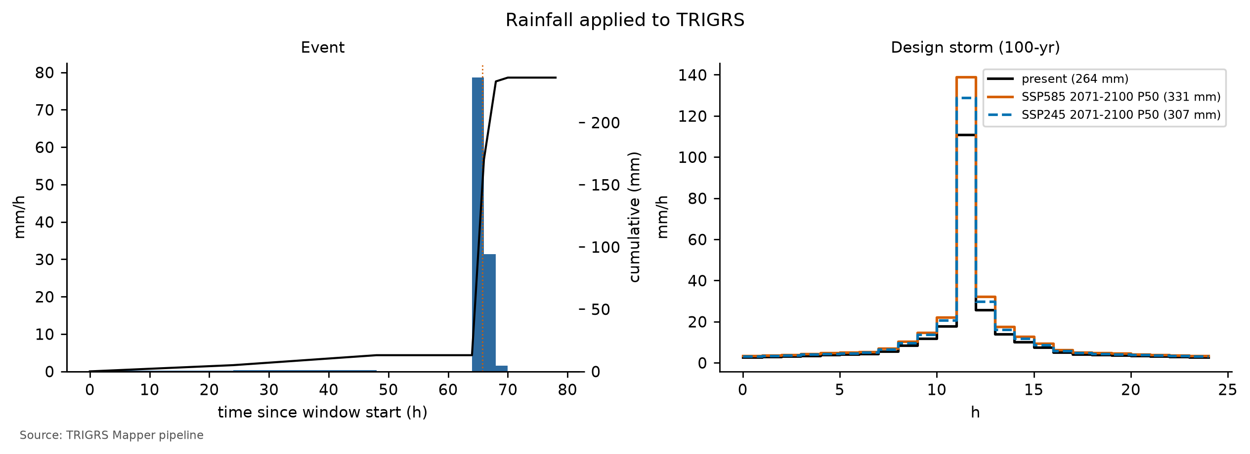
The rainfall over the window is very uncertain — from 131–147 mm in the outer ring to 220–260 mm at the storm core (Table 8.1) —, and the hourly pattern is constructed, not observed. The minimum (Bingen, 142 mm) and maximum (São Sebastião, 260 mm) scenarios of Table 8.14 are in chuva/evento_meta.json, but not in the format read by the sensitivity step; therefore the sensitivity to the scaling of the event rainfall has not been run for Petrópolis, and Table 8.36 has no rainfall rows (recommendation in Section 8.11). In the Morin watershed, the thresholds of Section 8.10 show that this uncertainty matters little for the model result: even the minimum scenario exceeds the 3-h and 6-h thresholds.

8.9.2 The 2022 inventory and source areas

There is no open official inventory of February 15, 2022: the municipal one (> 370 landslides, with failure and deposit mapped separately, cited by Ochi et al., 2022) is not public, the polygons of Alcântara et al. (2023) are only available on request, and the WorldView-3 mapping by Coelho Netto et al. (2022) was not published as data. The calibration reference is the set of Sentinel-2 candidates of exposed soil (pair November 29, 2021 × March 4, 2022, before the March 20 storm), by the base rule of project report 03 (dNDVI < −0.20, post-event NDVI < 0.35, and slope ≥ 15°), in the “clean” variant (objects with at least 3 pixels), visually checked on the 2-m CBERS-4A image (Figure 8.1). They are preliminary candidates, not validated against a field inventory.

TRIGRS predicts where a failure starts, but a scar polygon also includes the runout path and the deposit. The comparison therefore uses only the source area, approximated by the upper third, by elevation on the 10-m DEM, of each polygon:

• positives: 30-m cells centered in the source area with β ≥ 10° (at least one per scar);
• excluded: the rest of each polygon, dilated by one cell; the invalid cells of the Sentinel-2 mask (cloud, shadow, water); and the urban fabric (MapBiomas 2015, class 24), where vegetation was already sparse and dNDVI does not detect landslides;
• negatives: the remaining cells of the window.

This leaves 105 scars in the window, with 128 source cells against 22,906 negatives. The imbalance is huge — the source areas are a tiny fraction of the window —, which is why the calibration uses metrics that weigh both groups equally, instead of the overall accuracy (which would be high for an all-stable map).

8.9.3 Performance metrics

Each run is summarized by the confusion matrix, in cells, between the minimum FS of the event (unstable if FS < 1) and the inventory: true positives (TP, unstable source area), false negatives (FN, stable source area — omission), false positives (FP, unstable outside the scars — false alarm), and true negatives (TN). The minimum FS, however, does not tell when the cell became unstable. Each calibration run therefore also records the FS at the end of the two antecedent days, right before the storm, and splits the unstable source areas into already unstable before the event and triggered by the event (FS ≥ 1 before and FS < 1 after; TP_defl). With n = TP + FN + FP + TN:

\[ \begin{aligned} \text{TPR} &= \frac{TP}{TP+FN},\qquad \text{FPR} = \frac{FP}{FP+TN}\\[4pt] \text{MSR} &= \frac{\text{TPR} + (1-\text{FPR})}{2},\qquad \text{TSS} = \text{TPR} - \text{FPR}\\[4pt] \text{TPR}_{defl} &= \frac{TP_{defl}}{TP+FN},\qquad \text{TSS}_{defl} = \text{TPR}_{defl} - \text{FPR}\\[4pt] \text{MSR}_{defl} &= \frac{\text{TPR}_{defl} + (1-\text{FPR})}{2}\\[4pt] \kappa &= \frac{p_o - p_e}{1-p_e},\qquad p_o = \frac{TP+TN}{n}\\[4pt] p_e &= \frac{(TP+FP)(TP+FN) + (FN+TN)(FP+TN)}{n^2}\\[4pt] \text{LR}_k &= \frac{\text{fraction of source cells with FS in class } k}{\text{fraction of evaluated cells with FS in class } k} \end{aligned} \tag{8.11}\]

• TPR (hit rate) and FPR (false-alarm rate) measure the two errors separately. The MSR (modified success rate; Huang & Kao, 2006) is the mean of TPR and the hit rate of the negatives (1 − FPR): it is 0.5 for a map with no discriminating power and 1 for a perfect map, without being dominated by the huge number of negatives.
• Triggered TPR, MSR, and TSS (subscript defl, from deflagrado, “triggered”): the same formulas, but only the triggered scars count as hits. If the model has a source area unstable before the event, the place is right but the timing is wrong, and it counts as an omission; any unstable cell outside the scars, before or during the event, is a false alarm. The triggered MSR has been the calibration objective since decision D21, and the triggered TSS is the skill criterion (see below).
• TSS = TPR − FPR (0 = chance) and Cohen’s kappa (Cohen, 1960), which discounts the agreement expected by chance; with such rare source areas, kappa stays close to zero even for reasonable maps.
• AUC: area under the ROC curve (Fawcett, 2006), traced by varying the FS threshold with the score −FS (lower FS = more unstable). It measures the ranking of the cells, not only the cut at FS = 1: 0.5 = chance; 1 = perfect.
• LRclass (Park et al., 2013): likelihood ratio by FS class (< 1; 1–1.3; 1.3–1.5; 1.5–2; ≥ 2, the classes of the maps). LR > 1 means the class holds more source areas than area; a good model has a high LR in the FS < 1 class and a low one in the FS ≥ 2 class.
• Auxiliary criteria: unstable fraction of the window; ratio between unstable area and source area; median Z_cr in the unstable source areas, which should fall within 1–2.5 m, the depth of shallow failures in the region; rate of detected scars (at least one cell with FS < 1 in the source area); and the unstable fractions before the event, used as filters in the selection. The distance to the perfect point of the ROC curve, D2PC = √((1 − TPR)² + FPR²) (Formetta, Capparelli & Versace, 2016), is kept as a check.

8.9.4 Unstable before the rain: why the total MSR is not enough

TRIGRS starts from a steady initial condition — the initial water table and the background infiltration (Section 8.8) — and adds the effect of the rainfall to it. If this condition already leaves a cell with FS0 < 1, the model declares it unstable before the event, although the slopes that failed in 2022 were standing until the storm. In the calibration runs, almost all the instability before the storm comes from this initial condition: it comes neither from the rainfall of the two antecedent days (13 mm at Itamarati-SE) nor from the non-convergence of the series, a numerical problem measured separately (Section 8.8).

With the total MSR as the objective, this opens a shortcut. A parameter set weak enough to leave many steep slopes unstable already at t = 0 hits several source areas without the rain doing anything: the MSR goes up, but the hit is in the right place at the wrong time. In the partial test that led to decision D21, the winners by total MSR in Nova Friburgo and Teresópolis had exactly this profile, and in the full calibration it recurs in all three cases: in Petrópolis, the sample with the highest total MSR has most of its event’s unstable cells already unstable before the storm. The full calibration is therefore selected by the triggered MSR, with filters that require stable slopes before the event — as in the studies that calibrate TRIGRS with event inventories (Zieher et al., 2017; Schilirò, Esposito & Scarascia Mugnozza, 2015).

8.9.5 Latin hypercube search and selection (D21)

The parameters are not adjusted one by one: the calibration varies ten multipliers that scale the a priori values in all zones at once, preserving the spatial pattern of the parameterization (Equation 8.7; report 04, §10.3).

Table 8.30: Calibration multipliers: Latin hypercube ranges (150 samples; parameter table §10.3), a priori values and the best sample (lhs_0014). θ_s and G_s stay at their central values (γ_s derived). A priori rizero: the rate suggested by the antecedent rainfall capped to the recommended range (as in params.parametrizar). f_NA is an effective parameter (wetness left by the previous rains), not a measured water table; the volumes hold for that initial condition.

Multiplier	Acts on	LHS range	Scale	A priori	Calibrated
mc	effective cohesion c′	0.5–2	linear	1.00	0.78
mtanφ	tan φ′	0.85–1.15	linear	1.00	1.12
mKs	saturated conductivity Ks	0.1–10	logarithmic	1.00	4.22
rD0 (m)	diffusivity D0 = rD0·Ks	10–500	logarithmic	200	46
mα	Gardner α (unsaturated)	0.5–2	logarithmic	1.00	0.60
mz	soil thickness zmax	0.6–1.4	linear	1.00	0.88
kz (1/°)	decay of zmax with slope	0.025–0.045	linear	0.0347	0.0410
mCr	root cohesion Cr	0–1.5	linear	1.00	0.74
rizero (m/s)	initial (steady) infiltration	1 × 10⁻⁹ – 5 × 10⁻⁸	logarithmic	2.26 × 10⁻⁸ (antecedent)	1.04 × 10⁻⁸
fNA	initial water table = fNA·zmax	{0.5, 0.75, 1}	discrete	1.00	0.50

The Latin hypercube (McKay, Beckman & Conover, 1979) splits the range of each multiplier into n intervals of equal probability and draws exactly one sample in each interval, combining the intervals of the ten dimensions at random: with few runs, each range is covered from end to end. K_s, r_D0, α, and rizero vary on a logarithmic scale, and f_NA is discrete. The seed (20261031) is the same in the three cases, which generates the same set of samples in Nova Friburgo, Teresópolis, and Petrópolis and makes the rankings comparable in the cross-validation. The full run uses 150 samples (D20) plus the a priori run (multipliers equal to 1, water table at the base of the soil, and rizero from the antecedent rainfall).

Selection (decision D21). The choice is made in stages, all recorded in calibracao.json (Table 8.32):

1. Filters, never relaxed. A sample is only accepted if, before the event, at most 1% of the evaluated cells and at most 5% of the source cells are unstable; if at most 30% of the event’s unstable cells were already unstable before it; and if it triggers at least 5% of the source cells (triggered TPR ≥ 0.05). The limits come from studies that calibrate TRIGRS with event inventories: Zieher et al. (2017) accepted at most 0.5% of the catchment unstable at t = 0 and up to 4.9% of the landslides already unstable at the start; Schilirò, Esposito & Scarascia Mugnozza (2015) raised the cohesion until only 0.04% of the cells were unstable before the event. The margin up to 1% allows for the 30-m cells and the two antecedent days. The last filter requires minimum skill and excludes the null model: with no unstable cell at all, it has a triggered MSR of 0.5 and would win whenever the other samples miss more than they hit.
2. Numerical validity. At most 1% of cells without convergence of the series; this filter is only dropped if no sample meets it.
3. Auxiliary constraints, relaxable. Median Z_cr in the unstable sources between 1 and 2.5 m, unstable area up to 3 × the source area, and AUC ≥ 0.70. If no filtered sample meets all of them, they are dropped cumulatively, in this order, until at least one sample is left.
4. Objective. Among the remaining samples, the one with the highest triggered MSR wins. The 10 best form an ensemble: the susceptibility of each cell is the fraction of ensemble runs with FS < 1, and the AUC of this map is also reported (Raia et al., 2014).

In Petrópolis, the AUC ≥ 0.70 constraint is out of reach: the AUC of the 150 hypercube samples lies in the range 0.53–0.61, and no filtered sample meets all three auxiliary constraints (Table 8.32). The cumulative relaxation drops the median Z_cr and the unstable area with no sample left, and only when the AUC is dropped as well do the 18 samples of the filters come back: the choice rests on the filters and the objective (constraints relaxed: median Z_cr, unstable area and AUC). This is why the winner may have an unstable area far above 3 × the source area, as shown below.

trigrs_mapper.calibration (illustrative excerpt)

from trigrs_mapper.calibration import amostras_lhs, faixas_calibracao, metricas, selecionar

amostras = amostras_lhs(150, 20261031, faixas_calibracao())  # same LHS design in the three cases
# each sample becomes a run on the 30-m window; for each run:
m = metricas(fs_min, zcr, inventario, area_celula=900.0, com_roc=True, fs_pre=fs_fim_antecedente)
# m["msr_deflagrado"], m["tpr_deflagrado"], m["frac_instavel_pre"], m["frac_fonte_instavel_pre"],
# m["frac_instaveis_pre_evento"], m["auc"], m["lrclass"], ...
restricoes = {                                          # configs/cases/petropolis.yaml (D21)
    "frac_instavel_pre_max": 0.01, "frac_fonte_instavel_pre_max": 0.05,   # filters
    "frac_instaveis_pre_evento_max": 0.3, "tpr_deflagrado_min": 0.05,     # filters
    "frac_nao_convergentes_max": 0.01,                                    # numerical validity
    "zcr_mediana_m": [1.0, 2.5], "area_instavel_max_x_fonte": 3.0, "auc_min": 0.70,  # relaxable
    "filtros": ["pre"], "ordem_relaxamento": ["zcr", "area", "auc"]}
escolha = selecionar(linhas, restricoes, objetivo="msr_deflagrado", top_n=10)  # best sample and top-10 ensemble

Table 8.31: Calibration in the 30 m window (31,185 cells; 105 scars, 128 source cells): a priori run × best of the 150 Latin hypercube samples (seed 20261031), selected by triggered MSR among the 18 feasible ones (relaxed constraints: median Z_cr, unstable area and AUC); 2nd and 3rd places in the last columns. Event rainfall 15 Feb 2022: 236.0 mm in 17 periods. “Before the event” = end of the antecedent period; a scar already unstable before counts as a miss in the triggered MSR. Filters are never relaxed; relaxable constraints are dropped in the order shown only if no sample meets them.

Metric	Criterion	A priori	Best (lhs_0014)	2nd (lhs_0029)	3rd (lhs_0106)
MSR = (TPR + TNR)/2	reference (criterion before D21)	0.49	0.53	0.52	0.51
Triggered MSR = (triggered TPR + TNR)/2	objective (maximum)	0.49	0.52	0.52	0.51
AUC (score = −FS)	≥ 0.70 (relaxable, 3rd; relaxed)	0.57	0.58	0.60	0.59
TPR (source areas with FS < 1)	n/a	0.00	0.26	0.05	0.11
Triggered TPR (FS ≥ 1 before, < 1 in the event)	≥ 0.05 (filter)	0.00	0.25	0.05	0.11
FPR (FS < 1 outside the scars)	n/a	0.02	0.21	0.02	0.08
TSS = TPR − FPR	n/a	−0.02	0.05	0.03	0.02
Triggered TSS = triggered TPR − FPR	skill: ≥ 0.05	−0.02	0.04	0.03	0.02
Cohen’s kappa	n/a	−0.01	0.00	0.01	0.00
Unstable fraction of the window (%)	n/a	2.0	20.6	2.5	8.5
Evaluated cells unstable before the event (%)	≤ 1% (filter)	0.02	0.60	0.00	0.03
Source cells unstable before the event (%)	≤ 5% (filter)	0.0	0.8	0.0	0.0
Event-unstable cells already unstable before (%)	≤ 30% (filter)	1.1	2.9	0.0	0.4
Cells without series convergence (%)	≤ 1% (relaxable filter)	1.99	0.00	0.00	0.00
Unstable area ÷ source area	≤ 3.0 (relaxable, 2nd; relaxed)	3.7	37.1	4.4	15.3
Median Zcr in unstable sources (m)	1.0–2.5 (relaxable, 1st; relaxed)	n/a	1.31	0.99	1.05
Scars detected	n/a	0 of 105 (0.0%)	27 of 105 (25.7%)	6 of 105 (5.7%)	11 of 105 (10.5%)
Top-10 ensemble AUC (fraction of runs with FS < 1)	n/a	n/a	0.53	n/a	n/a

Table 8.32: Calibration selection (D21 rule): samples left after each stage — filters that are never relaxed, a numerical-validity filter (dropped only if no sample meets it) and auxiliary constraints relaxed cumulatively in the order median Z_cr → unstable area → AUC until at least one sample is left; the choice is by triggered MSR. Failures per criterion: samples violating each criterion (a sample may violate several).

Stage	Criteria	Samples left	Failures per criterion
LHS samples with metrics	150 samples run	150	no metrics: 0
Filters (never relaxed)	≤ 30% of the event’s unstable cells already unstable before it; ≤ 1% of the evaluated cells unstable before the event; ≤ 5% of the source cells unstable before the event; triggered TPR ≥ 0.05	18	pre-event share of unstable cells: 60; evaluated cells unstable before the event: 54; source cells unstable before the event: 20; triggered TPR: 101
Numerical validity (relaxed only if nothing is left)	≤ 1% of cells without convergence of the series	18	numerical validity (series convergence): 22
Auxiliary constraints (all)	median Zcr between 1 and 2.5 m; unstable area ≤ 3× the source area; AUC ≥ 0.70	0	median Z_cr: 63; unstable area: 87; AUC: 150
Relaxing median Z_cr	unstable area ≤ 3× the source area; AUC ≥ 0.70	0	n/a
Relaxing median Z_cr and unstable area	AUC ≥ 0.70	0	n/a
Relaxing median Z_cr, unstable area and AUC	filters only	18	n/a
Choice	triggered MSR (maximum)	lhs_0014 (0.522)	top-3: lhs_0014, lhs_0029, lhs_0106

Table 8.33: Reasons for exclusion in the selection: criteria violated at the first stage that excluded the sample (calibracao.json → selecao → contagem_exclusao).

Reason for exclusion	Samples
triggered TPR	59
pre-event share of unstable cells + triggered TPR	19
pre-event share of unstable cells + evaluated cells unstable before the event + triggered TPR	12
pre-event share of unstable cells + evaluated cells unstable before the event + source cells unstable before the event	11
evaluated cells unstable before the event	11
pre-event share of unstable cells + evaluated cells unstable before the event	9
pre-event share of unstable cells + evaluated cells unstable before the event + source cells unstable before the event + triggered TPR	9
evaluated cells unstable before the event + triggered TPR	2

The best sample (lhs_0014) was chosen by the triggered MSR: triggered MSR = 0.52 (a priori: 0.49), with triggered TPR = 0.25 and FPR = 0.21. The total MSR is 0.53 (a priori: 0.49) and the AUC is 0.58 (a priori: 0.57); the sample detects 27 of the 105 scars (25.7%). Before the event, 0.60% of the evaluated cells and 0.8% of the source cells were already unstable, and 2.9% of the event’s unstable cells already were (a priori: 0.02% and 1.1%); 0.00% of the cells did not converge. The unstable fraction of the window goes from 2.0% (a priori) to 20.6%, or 37.1 times the source area (auxiliary limit: 3), and the median Z_cr in the unstable sources is 1.31 m.

The selection stages left: 150 with metrics → 18 after the filters → 18 with numerical validity → 0 with the auxiliary constraints → 0 relaxing median Z_cr → 0 relaxing median Z_cr and unstable area → 18 relaxing median Z_cr, unstable area and AUC (Table 8.32; filters dropped: none). Only 18 of the 150 samples passed the filters, and, among them, the minimum triggered TPR was the most violated (Table 8.33). The three best by triggered MSR are lhs_0014 (0.522); lhs_0029 (0.515); lhs_0106 (0.512): the gap between the 1st and the 2nd (0.007) is small, but the three draw very different maps — the unstable fraction of the window ranges from a few percent to about one fifth of it (Table 8.31). The ensemble of the 10 best has AUC = 0.53, below the best sample and close to chance: samples that nearly tie by the criterion miss in different places, and their average does not rank the scars any better. Table 8.34 shows how the minimum FS of the event ranks the source areas.

Table 8.34: Likelihood ratio by FS class (LRclass; Park et al., 2013) of the event minimum FS in the 30 m window: LR = fraction of the scar source cells in the class ÷ fraction of the evaluated cells in the class (LR > 1: class enriched in scars). Area and scars in % of the evaluated cells and of the source cells.

FS class	A priori: area (%)	A priori: scars (%)	A priori: LR	Best (lhs_0014): area (%)	Best: scars (%)	Best: LR
FS < 1	2.0	0.0	0.00	20.6	25.8	1.25
1 ≤ FS < 1.3	9.8	10.2	1.03	25.3	31.2	1.24
1.3 ≤ FS < 1.5	10.4	13.3	1.28	8.1	8.6	1.06
1.5 ≤ FS < 2	28.4	35.2	1.24	25.0	25.8	1.03
FS ≥ 2	49.3	41.4	0.84	21.0	8.6	0.41

In the best sample, the FS < 1 class has LR = 1.25 (a priori: 0.00) and the FS ≥ 2 class, LR = 0.41 (a priori: 0.84). The critical classes (FS < 1.3) hold only slightly more source areas than area, and the FS ≥ 2 class holds far fewer: the minimum FS separates the very stable slopes but hardly distinguishes the scars within the critical classes — hence the low AUC.

ImportantSkill flag: in Petrópolis, the volumes are a scenario

D21 requires a minimum skill from the calibrated model: triggered TSS ≥ 0.05 and AUC ≥ 0.60. The best sample has triggered TSS = 0.04 and AUC = 0.58. Flag sem_habilidade (no skill): yes (no skill (triggered TSS 0.04 < 0.05; AUC 0.58 < 0.60): volumes presented as a scenario).

By Equation 8.11, triggered TSS = 2 · triggered MSR − 1: the 0.05 minimum is equivalent to a triggered MSR ≥ 0.525. None of the 150 samples gets there — the chosen one is already the sample with the highest triggered MSR in the whole hypercube —, nor does the regional sample lhs_0019, chosen in Nova Friburgo and in Teresópolis, which in Petrópolis passes the filters and enters the ensemble of the 10 best, but stays at the a priori level. Against the 2022 scar candidates, the calibration barely separates the failures from the rest of the window better than chance: the chosen configuration is stable — it passes the filters — but it is not a calibration.

The two results that seemed to indicate skill outside this reference do not demonstrate it. Transferred to the Vale do Cuiabá, the configuration outperforms the a priori run and meets both D21 minimums, but that window covers 66.5% of the calibration window and 96.2% of the cells of the watershed of Teresópolis, and it uses the 2011 Teresópolis rainfall: it tests the configuration in the Teresópolis area, not in Petrópolis nor with the 2022 rainfall. On the 2022 window re-evaluated at 10 m, the minimums are also reached, but mainly because, at that resolution, the same set makes less of the window unstable (cross-validation and sensitivity, below). The reference matters — preliminary Sentinel-2 candidates, detected by dNDVI, with the urban fabric excluded (D16) and scars that are small for the 30-m cell —, but the lack of skill cannot be attributed to it alone: with the central 2022 rainfall, the model puts 22.1% of the Morin watershed at FS < 1, where the screening found almost no scars; that is, it overestimates the instability (specificity test, below). The flag stays: the volumes of sections 8.10 and 8.11 are scenarios, that is, what this configuration produces with each rainfall, and not calibrated predictions. Recalibrating with the 2022 municipal inventory remains the priority, because it separates what comes from the reference from what comes from the model, but it does not guarantee skill: if the excess of unstable area persists, the cause lies in the parameters, the soil thickness, or the rainfall (Section 8.11). Remember also that V_d* is governed by V_dy2, which does not depend on TRIGRS, for all return periods and scenarios (Section 8.10).

Before the event, in the calibrated run. In the event run with the chosen configuration, 0.60% of the evaluated cells of the window were unstable before the storm, and 2.9% of the event’s unstable cells already were; the triggered MSR is 0.52, against a total MSR of 0.53. Both fractions are below the filters (1% and 30%): the model’s hits come from failures that the storm triggered, not from the initial condition.

8.9.6 Cross-validation: from Alto da Serra to the Vale do Cuiabá

The cross-validation applies the multipliers calibrated in Petrópolis to another window, with another rainfall and another inventory: the Vale do Cuiabá, in Itaipava, hit by the debris flow of January 2011 (Section 8.1). There the reference is the 2011 inventory of Marc et al. (2018) and Emberson et al. (2022), shifted +15 m E and −75 m N to match the Landsat images (decision D17), with the reconstructed rainfall of the Teresópolis event and the pre-event GLAD 2010 land cover. The MSR obtained with the Petrópolis multipliers is compared with that of the a priori run in the Vale do Cuiabá itself (Table 8.35).

Table 8.35: Cross-validation: multipliers calibrated in Petrópolis applied to another inventory and event, compared with the a priori run at the target, with the best sample of the target’s own calibration (target MSR, same window) and with the rank among the target’s Latin hypercube samples (by MSR and by triggered MSR, the D21 criterion).

Origin → target (rainfall)	Scars (source cells)	Transferred MSR	A priori MSR	Target MSR	Triggered MSR: transferred / a priori / target	AUC transferred / a priori	Rank in the target LHS (MSR; triggered MSR)
Petrópolis → Cuiabá Valley, Jan 2011 (D16) (rainfall of Teresópolis)	356 (709)	0.54	0.52	n/a	0.54 / 0.52 / n/a	0.72 / 0.76	n/a; n/a

The Petrópolis multipliers give MSR = 0.54 in the Vale do Cuiabá, against 0.52 for the a priori run (difference of +0.019), with AUC of 0.72 (a priori: 0.76). By the D21 criterion, the transferred triggered MSR is 0.54, against 0.52 a priori (difference of +0.016). Since the Vale do Cuiabá has no calibration of its own, there is no target ranking.

Both differences are positive, and the transfer meets the D21 skill minimums: with triggered TSS = 2 · triggered MSR − 1, the transferred triggered MSR corresponds to a triggered TSS above 0.05, and the AUC stays above 0.60 — while the a priori run does not reach the triggered-TSS minimum. The Petrópolis configuration hits more scars than the a priori run, and the gain comes from the cut at FS = 1, not from the ranking: the transferred AUC is below the a priori one.

Why this validation is not independent. To test Petrópolis, the validation would need a place, a rainfall, and an inventory unrelated to the calibrations. The Vale do Cuiabá window does not meet this: it extends over the Teresópolis area — it covers 66.5% of the Teresópolis calibration window and 96.2% of the cells of the Teresópolis watershed —, it is forced by the reconstructed 2011 Teresópolis rainfall, and it uses the same Marc et al. (2018) inventory as the Teresópolis calibration (Teresópolis chapter). What it measures is whether the Petrópolis configuration works in the Teresópolis area, with the 2011 event, not whether it works in Petrópolis or with the 2022 rainfall. The “skill in the Vale do Cuiabá” is, to a large extent, skill in the Teresópolis area, and it does not allow attributing the lack of skill in Petrópolis to the preliminary 2022 inventory alone. The test of the configuration in Petrópolis, with the 2022 rainfall, is that of the Morin watershed (below), and there the model overestimates the instability.

The validation with the March 20, 2022 storm, planned in decision D16 (Section 8.1), has not been run yet: it requires separating the March scars from the February ones (the Sentinel-2 pair November 29, 2021 × April 23, 2022 mixes the two events) and remains a recommendation (Section 8.11). It would be the first validation of the configuration in Petrópolis with another rainfall.

8.9.7 Where the model hits and where it misses

Figure 8.28 shows the minimum FS of the event over the window, with the calibrated configuration, and the classification of the cells. In the event run, triggered MSR = 0.52 (triggered TPR = 0.25), total MSR = 0.53, AUC = 0.58, TPR = 0.26, and FPR = 0.21, with 27 scars detected (25.7%). Read the map looking for patterns: false alarms in continuous bands of steep slopes indicate parameters too weak (or an initial water table too high) for those slopes; scattered omissions are usually small scars, which the 30-m cell does not resolve, or areas where the actual rainfall exceeded that of the central scenario.

Figure 8.28: Minimum FS of the February 15, 2022 event over the calibration window (30 m) with the calibrated configuration (left) and the comparison with the source areas of the Sentinel-2 scars (right): hits (source area with FS < 1), omissions (source area with FS ≥ 1), and false alarms (FS < 1 outside the scars). The metrics of the run are in the title.

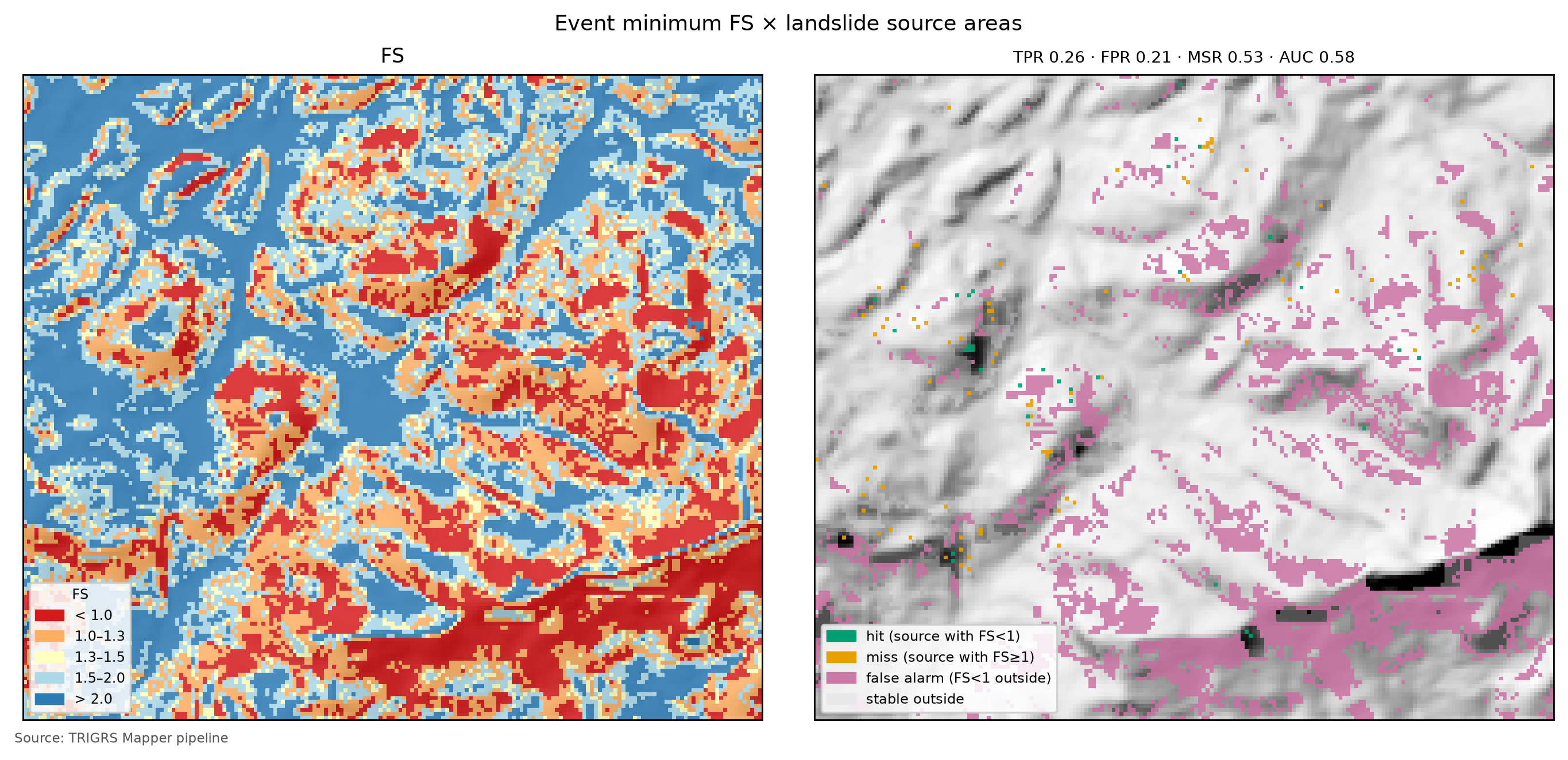
Figure 8.29 compares the ROC curves of the a priori run, the best sample, and the ensemble. A curve hugging the diagonal means that ranking the cells by FS does not separate the source areas better than a random draw; the more the curve rises on the left, the better.

Figure 8.29: Calibration ROC curves (score = −FS): a priori run, best sample, and ensemble of the best samples (score = fraction of runs with FS < 1), with the AUC of each. The diagonal is the performance of a random draw.

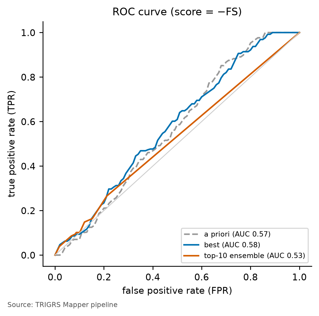
Does FS rank better than slope? The AUC does not require a physical model: any quantity that grows with the chance of failure ranks the cells, and the simplest is slope itself. With the same positives and negatives of the window, the AUC of slope alone is 0.58, and that of the calibrated FS, 0.58: in Petrópolis, both stay close to chance. In the other cases, slope even outperforms FS (0.70 vs. 0.66 in Nova Friburgo; 0.85 vs. 0.76 in Teresópolis). This is not a flaw of the calibration but a limit of what FS knows about space: in Equation 8.9, the friction and cohesion terms depend on the slope δ; so does the zmax of Equation 8.10; and the multipliers scale all zones alike. The where of FS is, to a large extent, the where of slope.

What slope does not tell is when the hillslope fails — it does not change with the rainfall — nor how much material is released. A static map has no triggered cells: all its hits would already be there before the rain, and its triggered MSR could not exceed 0.5. The value of TRIGRS in the coupling therefore lies in the triggering over time — the rainfall that brings the hillslopes to failure from the initial condition, measured by the triggered metrics, the thresholds, and the design curves — and in the volume, through the failure depth and the connection to the drainage (Section 8.10), not in the spatial ranking: the FS map must not be read as a susceptibility map better than the slope map.

Specificity test in the Morin watershed. The watershed of the reference point had almost no scars in 2022: the Sentinel-2 screening found no newly exposed soil with the base rule and only 1,000 m² with the calibrated rule (Table 8.19). Run at 10 m with the central event rainfall and the 2015 land cover, the calibrated configuration puts 22.1% of the watershed at FS < 1 (17.06 ha), of which 22.0% of the watershed is triggered by the rain; 0.17% of the watershed (13 cells) already has FS0 < 1. The model overestimates the instability in Morin: the area triggered in the event, 22.0% of a 0.771-km² watershed, is about two orders of magnitude above the ~0.1 ha of newly exposed soil found by the screening. The rainfall over the watershed is unknown and may have been lower than in the central scenario (Section 8.5.7), but that does not explain the difference: by the watershed thresholds, even the minimum event scenario would bring more than 5% of it to failure (Table 8.41). The specificity test repeats, in the design watershed, the excess of unstable area seen on the window, where the unstable area is 37.1 times the source area.

8.9.8 Sensitivity

The sensitivity analysis varies one factor at a time around the calibrated configuration, on the 30-m window, and measures two effects: on the window metrics (MSR, triggered MSR, and AUC) and on the event volume in the watershed (V_dep of all unstable cells inside the watershed mask; Section 8.10). The factors cover the largest uncertainties of the case:

• initial water table: scenarios d = 1 to 10 m (D6) and fractions 1, 0.75, and 0.5 of zmax;
• thickness: alternative zmax models (DeRose, uniform 1.25 and 2 m, linear, and “regolith”);
• strength and permeability: K_s × 0.1 and × 10, c′ × 0.5 and × 2, tan φ′ × 0.85 and × 1.15 (the limits of the ranges of the parameter table);
• infiltration: effective rainfall by SCS-CN (potential infiltration P − P_e, AMC II), saturated model, and hydro flow direction;
• resolution: the event in the watershed at 30 and at 10 m and, in the full run, the calibrated configuration re-evaluated on the window at 10 m (D12).

Table 8.36 lists the 27 variations of the full run (mode: full). At the base, the MSR is 0.53, the triggered MSR, 0.52, and the AUC, 0.58.

Table 8.36: One-at-a-time sensitivity around the calibrated configuration (full calibration, sample lhs_0014), in the 30 m window: event V_dep in the watershed (all unstable cells, watershed mask in the window) and MSR/AUC in the window; Δ relative to the base (on the base row, the triggered MSR in parentheses). Last rows: the event in the watershed at 10 m × 30 m (same parameters and rainfall).

Variation	Vdep (m³)	ΔVdep (%)	MSR	ΔMSR	Δ triggered MSR	AUC
base configuration	185,080	n/a	0.53	n/a	(0.52)	0.58
initial water table d = 2 m	44,530	−75.9	0.49	−0.031	−0.027	0.58
initial water table d = 3 m	44,530	−75.9	0.49	−0.031	−0.027	0.57
initial water table d = 1 m	93,373	−49.5	0.50	−0.028	−0.024	0.59
initial water table d = 4 m	44,530	−75.9	0.49	−0.031	−0.027	0.57
initial water table d = 5 m	44,530	−75.9	0.49	−0.031	−0.027	0.57
initial water table d = 6 m	44,530	−75.9	0.49	−0.031	−0.027	0.57
initial water table d = 7 m	44,530	−75.9	0.49	−0.031	−0.027	0.57
initial water table d = 8 m	44,530	−75.9	0.49	−0.031	−0.027	0.57
initial water table d = 9 m	44,530	−75.9	0.49	−0.031	−0.027	0.57
initial water table d = 10 m	44,530	−75.9	0.49	−0.031	−0.027	0.57
initial water table = 1·zmax	44,530	−75.9	0.49	−0.031	−0.027	0.57
initial water table = 0.75·zmax	118,557	−35.9	0.51	−0.016	−0.012	0.58
initial water table = 0.5·zmax	185,080	0.0	0.53	0.000	0.000	0.58
uniform zmax of 1.25 m	135,600	−26.7	0.51	−0.013	−0.029	0.58
uniform zmax of 2.0 m	265,755	+43.6	0.54	+0.011	−0.016	0.58
zmax: DeRose model	175,304	−5.3	0.49	−0.032	−0.044	0.57
zmax: linear (4 → 0.3 m) model	189,188	+2.2	0.51	−0.014	−0.022	0.58
zmax: regolith (BDTICM) model	146,965	−20.6	0.52	−0.008	−0.062	0.57
Ks × 10	32,450	−82.5	0.50	−0.026	−0.026	0.58
c′ × 0.5	289,614	+56.5	0.55	+0.022	−0.006	0.60
c′ × 2	5,795	−96.9	0.51	−0.018	−0.014	0.57
Ks × 0.1	87,214	−52.9	0.50	−0.029	−0.029	0.57
tan φ′ × 0.85	289,546	+56.4	0.56	+0.035	+0.016	0.58
saturated model	82,881	−55.2	0.49	−0.035	−0.074	0.60
tan φ′ × 1.15	89,975	−51.4	0.49	−0.032	−0.028	0.58
infiltration P − Pe (SCS-CN, AMC II)	40,028	−78.4	0.49	−0.032	−0.032	0.57
flowdir = hydro	375,629	+103.0	0.55	+0.020	−0.046	0.58
watershed resolution 10 m × 30 m — all unstable cells	154,407 (30 m: 185,080)	−16.6	n/a	n/a	n/a	n/a
watershed resolution 10 m × 30 m — patch (D19 total, incl. FS0 < 1)	122,635 (30 m: 182,508)	−32.8	n/a	n/a	n/a	n/a

Figure 8.30: Tornado plot of the one-factor-at-a-time sensitivity: change (%) in the event V_dep in the watershed (all unstable cells inside the watershed mask, on the 30-m window; the value of the calibrated configuration is in the title) and effect of the watershed resolution (10 vs. 30 m), sorted by effect size. Bars to the right increase the volume.

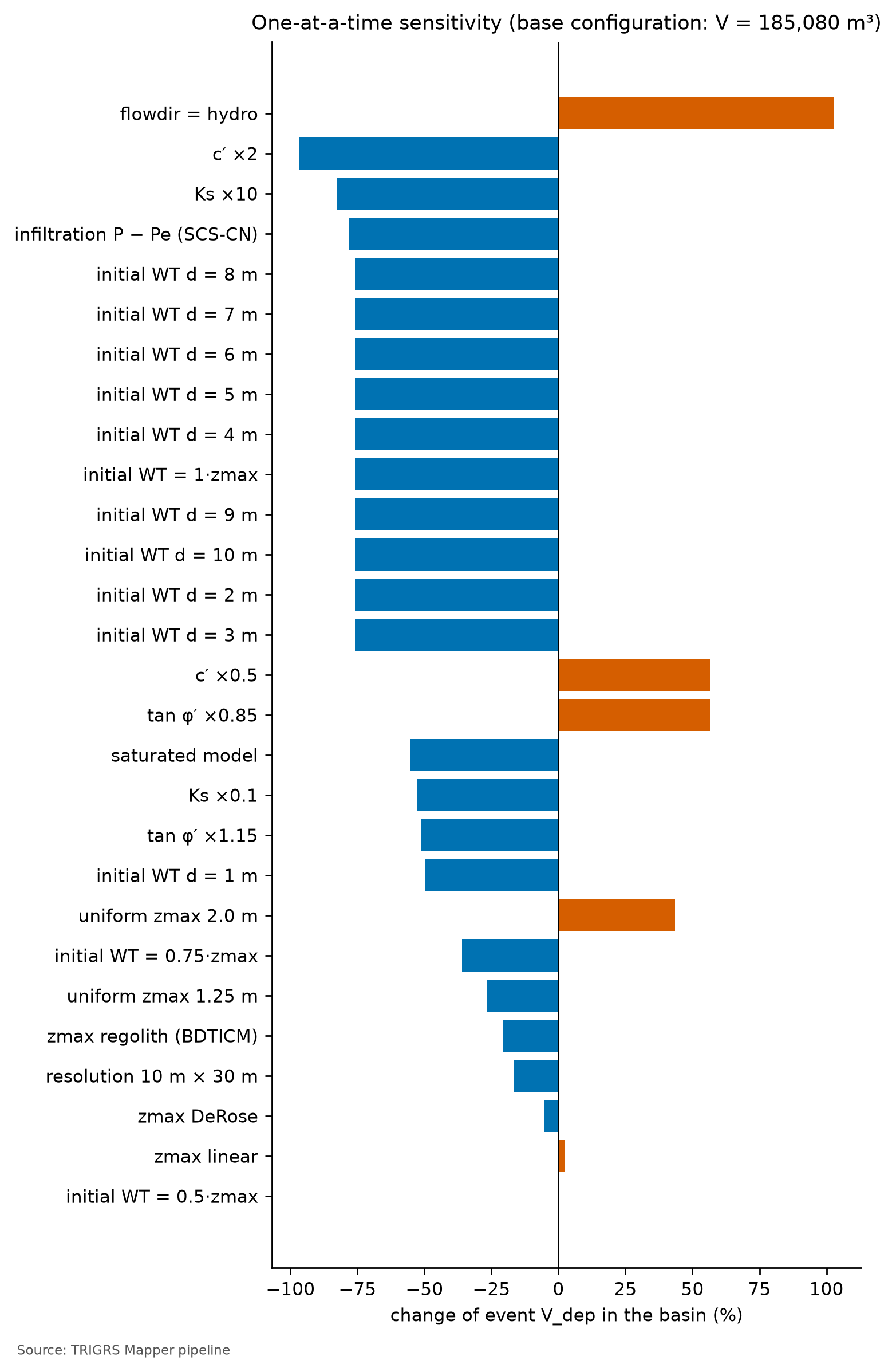
The factor with the largest effect on the event volume is flowdir = hydro (+103.0%): with hydro, TRIGRS allows higher pressure heads than with slope-parallel flow, and more slopes fail. Next come the cohesion (c′ × 2: −96.9%; c′ × 0.5: +56.5%), the conductivity (K_s × 10: −82.5%), the SCS-CN infiltration (−78.4%), and the initial water table at the base of the soil (−75.9%): with the parameter and model uncertainties, the event volume changes by tens of percent, nearly vanishes, or doubles. The window metrics barely move — the largest effect on the MSR is that of the saturated model (−0.035) —, that is, the calibration on the window hardly constrains the volume: one more reason to read it as a scenario.

For the triggered MSR, the largest effects come from the model choices: saturated model (−0.074), zmax from the regolith (−0.062), flowdir = hydro (−0.046), and the DeRose zmax (−0.044). In the saturated model, all the unstable cells of the event were already unstable before the storm, and all the failures count as omissions. Almost every variation worsens the triggered MSR; only tan φ′ × 0.85 improves it (+0.016), and it does so by leaving unstable before the event a part of the window larger than the D21 filters allow.

An initial water table at 1 m changes the volume by −49.5%, the MSR by −0.028, and the triggered MSR by −0.024; at 10 m (water table at the base everywhere in the watershed), by −75.9%, −0.031, and −0.027. The initial water table acts twice: on the rainfall still needed for failure and on the initial condition itself — a higher water table leaves more cells with FS0 < 1, which the total MSR would count as hits and the triggered MSR counts as omissions. On the window, all scenarios with d ≥ 2 m give the same result as the water table at the base of the soil (Table 8.36); only d = 1 m stands apart, because a water table at 1 m lies above the base in the cells with soil thicker than 1 m — colluvia and residual soil —, where Z_cr is larger and each unstable cell weighs more in the volume. These scenarios put the water table deeper than in the calibrated configuration (f_NA = 0.50) — except the 1-m one in the thickest soils, which lie on gentle slopes and do not fail in any of these scenarios —, and the volume falls in all of them.

Resolution. The same event run in the watershed at 30 and at 10 m gives almost the same unstable fraction (22.5 and 22.1%), but V_insitu of all unstable cells of 209,938 and 170,167 m³ (−18.9%). The difference is larger in the volume connected to the drainage (decision D19): the patch accounts for 98.6% of the V_dep of all unstable cells at 30 m and for 79.4% at 10 m (patch V_dep: 182,508 vs. 122,635 m³; −32.8%), for the reasons explained in Section 8.10.2. When the calibrated configuration is checked on the window itself, the metrics improve at 10 m: the MSR goes from 0.53 (30 m) to 0.57 (10 m), the triggered MSR from 0.52 to 0.57, and the AUC from 0.58 to 0.61. At 10 m, the configuration meets both D21 skill minimums (triggered TSS = 2 · triggered MSR − 1 above 0.05 and AUC ≥ 0.60), but this does not show that the lack of skill comes only from scars too small for the 30-m cell. The same set, calibrated at 30 m, makes only 14.8% of the window unstable at 10 m, against 20.6% at 30 m, and most of the improvement in the MSR and the triggered MSR comes from fewer false alarms, and only part of it from more hits. The calibrated parameters are not independent of resolution — at 10 m, the calibrated set also makes less of the window unstable in Nova Friburgo (6.0 vs. 7.9%) and in Teresópolis (2.6 vs. 4.7%) —, and the 10-m watershed of the event and design runs uses a set calibrated at 30 m. In the Morin watershed, the unstable fraction of the event hardly changes with resolution (above): with the 2022 rainfall, almost all the susceptible hillslopes of the watershed fail at both resolutions.

8.9.9 What the calibration says

1. No skill against the 2022 inventory. The best sample has triggered TSS = 0.04 and AUC = 0.58, below the D21 minimums, and none of the 150 samples reaches them: the flag does not come from the selection rule. It comes from confronting the model with the 2022 reference at 30 m, and the specificity test shows that the model overestimates the instability with the 2022 rainfall.
2. Right timing. The winner passes the filters: 0.60% of the evaluated cells and 0.8% of the sources unstable before the event, and 2.9% of the event’s unstable cells already unstable before it. By the total MSR, the choice would fall on a sample in which most of the event’s unstable cells were already unstable before the rain.
3. Partial physical plausibility. The median Z_cr in the unstable sources (1.31 m) falls within the range of shallow failures (1–2.5 m), but, since Z_cr = zmax in 100.0% of the unstable cells of the window, this checks the calibrated thickness model, not the hydrological response (Section 8.10). The unstable area is 37.1 times the source area (auxiliary limit: 3), and AUC ≥ 0.70 is out of reach (maximum of 0.61): the three auxiliary constraints were relaxed.
4. Validation not independent. In the Vale do Cuiabá, with the 2011 inventory, the same configuration outperforms the a priori run and meets the skill minimums (triggered MSR 0.54; AUC 0.72), but that window covers 66.5% of the window and 96.2% of the watershed of Teresópolis and uses the Teresópolis rainfall: it is a test in the Teresópolis area, not in Petrópolis nor with the 2022 rainfall. On the 2022 window re-evaluated at 10 m, the minimums are also reached (triggered MSR 0.57; AUC 0.61), mainly because, at 10 m, the set makes less of the window unstable (sensitivity, above).
5. Poorly identifiable. The top samples nearly tie (gap of 0.007) with very different maps, the ensemble is close to chance (AUC = 0.53), and the tornado plot changes the event volume by tens of percent — up to doubling it, with flowdir = hydro — with a minimal effect on the MSR: the calibration on the window hardly constrains the volume. For the triggered MSR, the model choices weigh more (saturated model and soil thickness).
6. Resolution. From the 30-m to the 10-m watershed, the patch V_dep of the event changes by −32.8%. On the window, the metrics improve at 10 m, but the set calibrated at 30 m makes less of the window unstable at that resolution (14.8 vs. 20.6%): the calibrated parameters depend on the resolution at which they are applied.
7. Slope ranks as well as FS. With the same positives and negatives, the AUC of slope alone (0.58) is at the level of that of the calibrated FS (0.58). TRIGRS does not improve the spatial ranking of the hillslopes; what it adds is the triggering over time and the volume (Section 8.10).

In short, the chosen configuration is stable before the event, but it does not fit the 2022 scar candidates, it overestimates the unstable area with the 2022 rainfall, and it does not rank the scars better than slope; the Vale do Cuiabá validation, which overlaps the Teresópolis area, does not demonstrate skill in Petrópolis. The Petrópolis volumes remain a scenario, and recalibrating with the 2022 municipal inventory remains the priority — to separate what comes from the reference from what comes from the model, with no guarantee that this will be enough to clear the flag (Section 8.11).

8.10 From TRIGRS to Vdy12

The traditional method left a gap in Petrópolis: V_dy12 by method “b” (zero-order thalwegs) assumes the watershed failing like Córrego D’Antas in 2011, whereas the 2022 screening found almost no failures inside it (Section 8.7.3). TRIGRS estimates, for each rainfall, which slopes fail and with what thickness. This section turns that into volume, as proposed in chapter 1 and as done in the example of chapter 5, with three project decisions: how to count the volume (D18), the criterion of connection to the drainage (D19), and the separation between the cells triggered by the rainfall and those already unstable at the initial condition (D21).

WarningRead the Petrópolis volumes as a scenario

Calibration skill flag (sem_habilidade, no skill): yes (no skill (triggered TSS 0.04 < 0.05; AUC 0.58 < 0.60): volumes presented as a scenario; Section 8.9). While it is raised, the volumes of this section show what the chosen configuration — stable before the event, but without skill in Petrópolis (the Vale do Cuiabá validation, which overlaps the Teresópolis area, does not demonstrate it) — produces with each rainfall; they are not calibrated predictions and, in the Morin watershed, they overestimate the 2022 failures. The design volume does not change because of this: for all return periods and scenarios, it is governed by V_dy2 (see below).

8.10.1 Three ways of counting the volume (D18)

\[ \begin{aligned} V_{insitu} &= \sum_{i\,:\,FS_i<1} A_{px}\,Z_{cr,i}\\ V_{dep} &= \sum_{i\,:\,FS_i<1} A_{px}\,Z_{cr,i}\,\frac{1-\theta_{s,i}}{1-\lambda}\\ V_{solto} &= \frac{V_{insitu}}{1-\lambda},\qquad \lambda = 0.4 \end{aligned} \tag{8.12}\]

• V_insitu is the intact soil above the failure surface. Since TRIGRS measures Z vertically, the prism above a slope-parallel failure has a volume of exactly A_px·Z_cr (normal thickness Z·cos δ times inclined area A_px/cos δ). It is directly comparable to V_dy11 and V_dy12 of the manual (B_d·D_e·L, measured in situ, with bulking neglected; GIDES manual, p. 34; NILIM TN 904) and to the method “a” variants of Table 8.19.
• V_dep is the main form, by conservation of solids: the in situ soil has porosity θ_s (that of the zone), so its solids occupy V_insitu·(1 − θ_s); deposited with the porosity λ = 0.4 of the manual (the K_v of Equation 8.6), the same solids occupy V_dep. When θ_s ≈ λ, V_dep ≈ V_insitu.
• V_solto (loose, bulked) is the convention of chapter 5, kept for comparison: it divides the in situ volume by 1 − λ as if the intact column had no voids. It is therefore an upper bound, 67% above V_insitu. In the synthetic example of chapter 5 the simplification does not change the lesson (the comparison with V_dy2); in a real design, it inflates the hillslope volume.

TipNumerical example: one 10-m cell

A cell of shallow soil over rock (θ_s = 0.45) with FS < 1 and Z_cr = 1.0 m (the cap of the shallow soil in the AR unit):

• V_insitu = 100 m² × 1.0 m = 100 m³ of intact soil;
• solids = 100 × (1 − 0.45) = 55 m³ → V_dep = 55 / (1 − 0.4) = 91.7 m³ of deposit;
• V_solto = 100 / (1 − 0.4) = 166.7 m³, 82% above V_dep.

In a colluvium (θ_s = 0.48) with Z_cr = 2.5 m: V_insitu = 250 m³, V_dep = 250 × 0.52 / 0.6 = 216.7 m³, and V_solto = 416.7 m³. In a talus deposit (θ_s = 0.38), V_dep ends up 3% above V_insitu, because this soil is less porous than the debris-flow deposit.

8.10.2 Connection to the drainage (D19)

Not every slope that fails feeds the debris flow at the reference point. The manual (§2.5.1.1) defines V_dy1 as the volume that can be converted into a debris flow, that is, the material that reaches the channel. Each volume form is therefore counted under three criteria of connection to the drainage network (cells with A ≥ 1 ha; Table 8.37).

Table 8.37: Criteria of connection of the TRIGRS volume to the drainage (trigrs_mapper.trigrs.volume).

Criterion	Cells counted	Role
todas (all)	all cells with FS < 1 in the watershed	upper bound (literal reading of method “a”: “slopes liable to fail”)
mancha (patch)	patches of unstable cells (8-neighborhood) that contain a channel cell or touch it	main: Vdy12* = patch Vdep (with D21, triggered cells only)
trajetoria (path)	cells whose D8 path to the channel runs only through unstable cells	lower bound

The three forms are computed for the three connectivities (nine volumes per run). The connection depends on the resolution: at 30 m, each cell covers 900 m², and neighboring unstable patches merge and touch the channel easily; at 10 m, the patches are smaller and more fragmented, and many remain isolated on the hillslopes. In the smoke test that motivated decision D19 (Petrópolis, TR 100), the patch gathered almost all the unstable volume at 30 m and only a small part of it at 10 m. In the full run, the calibrated configuration brings so many slopes to failure in the event that the patch gathers 98.6% of the V_dep of all unstable cells at 30 m and still 79.4% at 10 m (Section 8.9). The event and design volumes of this chapter use the 10-m watershed.

trigrs_mapper.trigrs.volume (illustrative excerpt)

from trigrs_mapper.trigrs.volume import calcular_volume_trigrs

# fs, zcr: TRfs_min and TRz_at_fs_min grids of the same instant (10-m watershed)
# canal: cells with A >= 1 ha; d8: directions in the TopoIndex scheme; theta_s: θs of each cell's zone
for conect in ("todas", "mancha", "trajetoria"):
    v = calcular_volume_trigrs(fs, zcr, area_celula=100.0, mascara_bacia=bacia, conectividade=conect,
                               drenagem=canal, direcoes=d8, lambda_porosidade=0.4, porosidade_solo=theta_s)
    print(conect, round(v.v_insitu_m3), round(v.v_dep_m3), round(v.v_solto_m3))
# D21: the pipeline repeats the count with FS < 1 only in the triggered cells (FS0 >= 1; suffix _defl)
# and only in the cells already unstable at t = 0 (FS0 < 1; suffix _inicial)

8.10.3 Triggered by the rainfall vs. unstable since t = 0 (D21)

The FS0 of Section 8.8 splits the unstable cells of each run into two groups: those triggered by the rainfall (FS0 ≥ 1 and minimum FS < 1) and those already unstable at t = 0 (FS0 < 1), which would fail with no rain at all. For each form and each connectivity, the pipeline then counts three volumes:

• triggered (suffix _defl): only the triggered cells — the patches and paths are formed by them alone, and the cells with FS0 < 1 act as a barrier in the connection to the channel;
• total (that of D19): all unstable cells, including those with FS0 < 1;
• initial share (suffix _inicial): only the cells with FS0 < 1, with the Z_cr of the run.

For todas, total = triggered + initial; for mancha and trajetoria the sum does not close, because merging the cells changes the patches and the paths. V_dy12* becomes the patch V_dep of the triggered cells only; the D19 total remains as a conservative upper bound, reported alongside, and the initial share (1 − V_dy12* ÷ total) is reported separately. There are three reasons (decision D21):

1. the initial share does not respond to the rainfall: it is the same for all return periods and scenarios, and adding it dilutes the response to climate change;
2. it would fail without rain: assigning it to the design storm mixes the initial condition with the effect of the storm;
3. the studies that calibrate TRIGRS with events avoid this instability in the calibration or exclude it from the count (Zieher et al., 2017; Schilirò, Esposito & Scarascia Mugnozza, 2015; Zhang et al., 2022), and none of those we consulted deliberately adds it to the volume.

The state at t = 0 also has a volume of its own, V0 — the patch V_dep formed only by the cells with FS0 < 1, with the Z_cr of t = 0 —, which depends neither on the return period nor on the climate.

8.10.4 The February 15, 2022 event in the watershed

Table 8.38: TRIGRS volumes of the February 15, 2022 event in the 10-m watershed (calibrated configuration, central rainfall, 2015 land cover, minimum FS of the event): three forms (D18) × three connectivities (D19), with the rainfall-triggered cells only and with all unstable cells (D19 total). In bold, the V_dy12* of the event by the D21 rule; the initial-share row counts only the cells with FS0 < 1. For “all”, total = triggered + initial share; for the other connectivities the sum does not close. State of the results: final — full.

Form	Cells	Path (lower bound)	Patch (main)	All
Vinsitu (m³)	triggered	9,937	134,099	169,067
Vinsitu (m³)	total (D19)	9,937	135,199	170,167
Vdep (m³)	triggered	8,644	121,626	153,398
Vdep (m³)	total (D19; upper bound)	8,644	122,635	154,407
Vdep (m³)	FS0 < 1 only (initial share)	0	0	1,008
Vsolto (m³)	triggered	16,562	223,499	281,779
Vsolto (m³)	total (D19)	16,562	225,332	283,612

In the event, the calibrated configuration puts 1,706 cells (17.06 ha, 22.1% of the watershed) at FS < 1, with a mean Z_cr of 1.00 m. Of these, 1,693 were triggered by the rainfall (22.0% of the watershed), and 0.8% were already unstable at t = 0; with the event land cover, 0.17% of the watershed (13 cells) has FS0 < 1. The V_dy12* of the event is 121,626 m³ (V_dep of the patch connected to the drainage, with the rainfall-triggered cells only (D21)); the D19 total, an upper bound, is 122,635 m³, with an initial share of 0.8%. Most of the unstable material lies in patches connected to the channel: the (total) patch V_dep is 79.4% of the V_dep of all unstable cells (Table 8.38). At t = 0, with no rain, the patch of the cells with FS0 < 1 is V0 = 0 m³ (all: 1,008 m³): these cells do not reach the channel on their own, and excluding the initial condition hardly changes the event volume.

Figure 8.31 shows where in the profile the failures form. With positive cohesion, the cohesion term of Equation 8.9 decreases with depth and the minimum FS tends to lie at the base of the soil. In Petrópolis this is more than a tendency: Z_cr = zmax in 100.0% of the unstable cells of the event in the watershed and in 100.0% of the unstable cells of the calibration window — the two distributions of Figure 8.31 coincide, and the failures always form at the contact with the base of the soil. In the shallow-soil cells, this puts Z_cr at the 1-m cap; in the colluvia, Z_cr is larger and each unstable cell is worth more volume. Most unstable cells sit at the 1-m cap or below it, at the lower edge of the range of the observed shallow failures (mean Z_cr of 1.00 m). The volume-per-cell map (Figure 8.32) is the Z_cr map — that is, the zmax map — of the unstable cells itself, multiplied by 100 m².

What this means for V_dy12*. If the failure always forms at the base of the soil, the rainfall decides which cells fail, when, and which of them connect to the channel, but not how thick the failure is: each unstable cell enters with A_px·zmax, and zmax comes from the thickness model of Equation 8.10 — the calibrated coefficients m_z = 0.88 and k_z = 0.0410/degree and the caps by unit, among them the 1-m cap of the AR3 unit, inherited from the 1:250,000 soil map. V_dy12* is thus the sum of A_px·zmax over the triggered cells connected to the channel, corrected for porosity (Equation 8.12): the hydrological part of the model picks the cells, and the thickness model gives the depth. It inherits that model and its uncertainty directly. Three consequences: (i) the median Z_cr, an auxiliary criterion of the calibration (Section 8.9), tests the coefficients of this model, not the hydrological response; (ii) the calibration on the window hardly constrains the thickness — in the tornado plot, a uniform zmax of 2 m changes the event V_dep by +43.6% and the triggered MSR by only −0.016, and a uniform 1.25 m, by −26.7% and −0.029 (Table 8.36) —, and only field measurements can pin it down (Section 8.11); (iii) more rainfall does not deepen failures that already form at the base of the soil, it only adds cells — which helps to understand the plateau of the design curves (below).

Figure 8.31: Critical depth Z_cr of the unstable cells of the event in the watershed (bars) and zmax of the same cells (outline). The shaded band is the 1–2.5 m depth of the shallow failures observed in the region; when the two distributions coincide, the failure forms at the contact with the base of the soil.

Figure 8.32: Mobilizable volume per cell in the event (m³ = 100 m² × Z_cr, in situ, all unstable cells), with the sum and the V_dy12* in the title. Isolated cells on the hillslopes enter the upper bound (all) but not V_dy12* (patch).

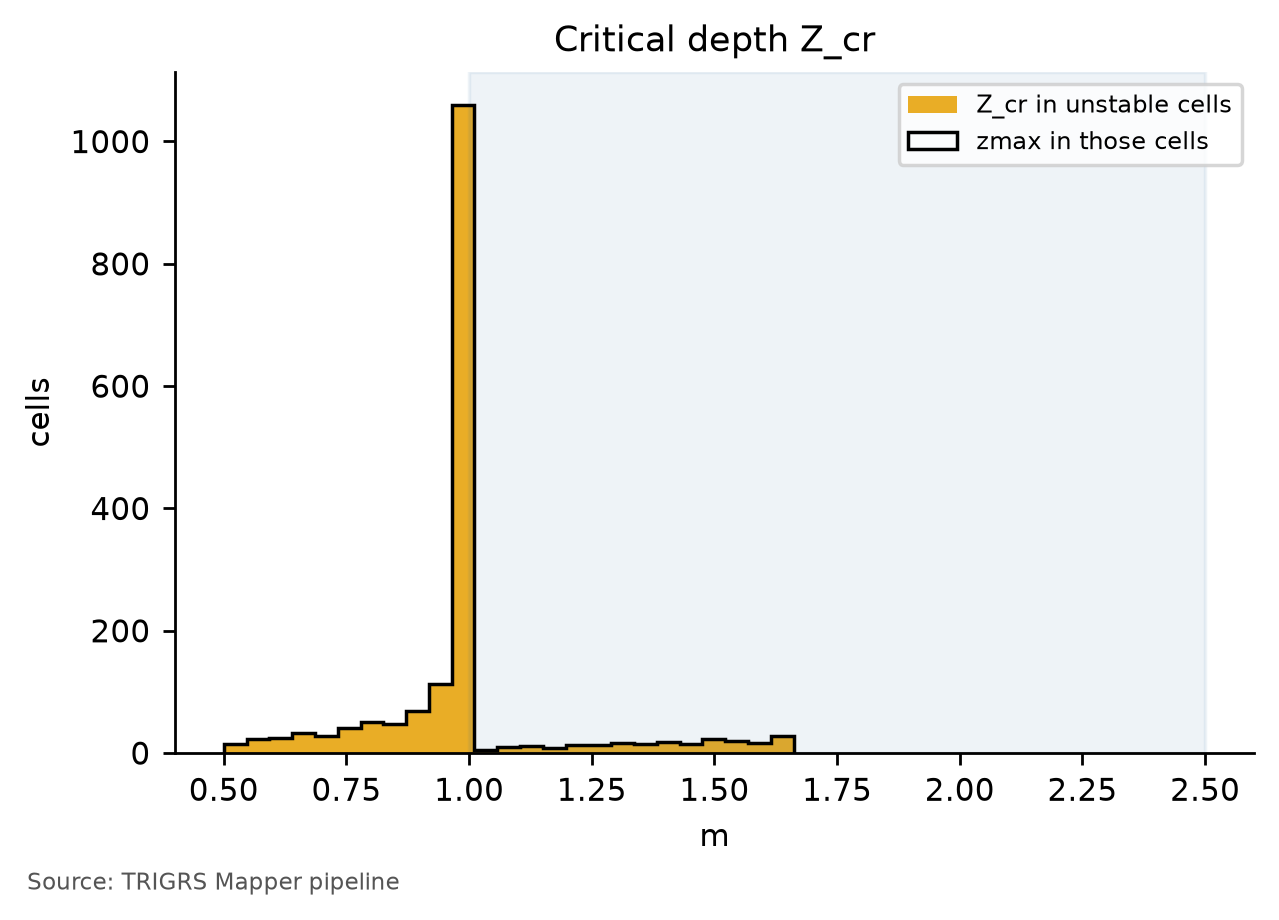
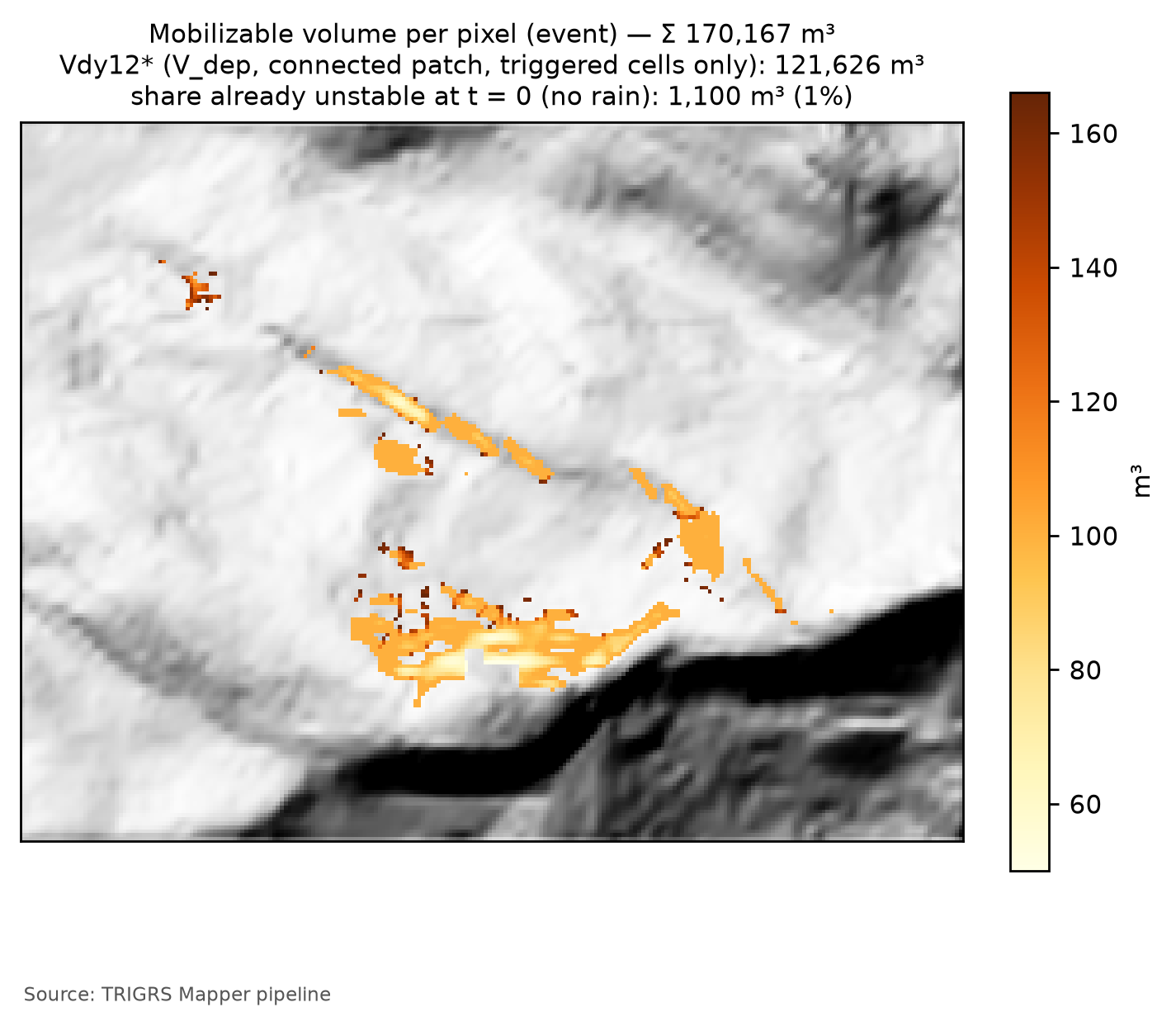
Comparison with 2022. Inside the watershed, Sentinel-2 indicated at most 1,000 m² of newly exposed soil after February 15, 2022 — 1,000 to 2,000 m³ with a thickness of 1 to 2 m (Table 8.19). The event V_dy12*, 121,626 m³, is about two orders of magnitude above that: the model overestimates the response of Morin to the central rainfall. A lower rainfall over the watershed, 2–2.5 km from the storm core (Section 8.5.7), would explain only part of the difference, because even the minimum event scenario exceeds the 3-h and 6-h volume thresholds of the watershed (Table 8.41). The event V_dy12* is already of the order of the plateau of the design curves (see below): for the model, the 2022 storm brought almost all the susceptible slopes of the watershed to failure. With the skill flag raised, this reinforces that the design volumes below are scenarios and that they tend to overestimate the failures.

8.10.5 Volume × TR curves at present and in the future

The design runs apply the 24-h hyetographs of Section 8.5.5 — at present and under the scenarios of Section 8.6 — to the 10-m watershed, with the current land cover (MapBiomas 2025) and the calibrated configuration. The full run covers 8 return periods (2 to 500 years) and 11 scenarios: the present; SSP2-4.5 and SSP5-8.5 in 2041–2070 (P50) and in 2071–2100 (P10, P50, and P90); and SSP1-2.6 and SSP3-7.0 in 2071–2100 (P50). The P10–P90 band is the spread among climate models of the rainfall change factor (Table 8.15), not a TRIGRS uncertainty. The calibrated initial water table and rizero are the same for all return periods and scenarios.

Table 8.39: Vdy12* (m³) by scenario and return period (columns, in years): V_dep of the patch connected to the drainage with the rainfall-triggered cells only (FS0 ≥ 1 at t = 0 and minimum FS < 1; D21), at present and under the climate scenarios (P10, P50 and P90 of the model ensemble). For the present, also the lower bound (continuous path to the channel), the D19 total (includes the cells already unstable at the initial condition; upper bound of Vdy12*), the initial share (patch formed only by the cells with FS0 < 1, which responds neither to the return period nor to the climate; not additive) and all unstable cells. State at t = 0: patch V_dep = 0 m³. 10 m watershed, land cover MapBiomas 2025, calibrated configuration.

Scenario / RP (yr)	2	5	10	25	50	100	200	500
present — path, triggered cells only (lower bound)	437	1,341	2,635	5,491	6,867	8,644	8,644	8,644
present — Vdy12* (patch, triggered cells only)	1,550	3,713	16,011	29,045	38,616	117,992	117,992	117,992
present — patch including cells unstable at t = 0 (D19 total; upper bound)	1,550	3,713	16,011	29,045	38,616	124,926	124,926	124,926
present — initial share (patch of the cells with FS0 < 1)	0	0	0	0	0	0	0	0
present — all unstable cells (literal reading of method a)	69,269	92,794	111,903	142,194	153,424	156,698	156,698	156,698
SSP1-2.6 2071–2100 P50	2,107	4,752	23,276	37,779	117,992	117,992	117,992	117,992
SSP2-4.5 2041–2070 P50	2,316	4,843	23,813	38,056	117,992	117,992	117,992	117,992
SSP2-4.5 2071–2100 P50	2,772	15,828	25,867	39,180	117,992	117,992	117,992	117,992
SSP2-4.5 2071–2100 P10	1,883	3,713	15,828	27,500	38,616	117,992	117,992	117,992
SSP2-4.5 2071–2100 P90	3,238	24,258	38,056	117,992	117,992	117,992	117,992	117,992
SSP3-7.0 2071–2100 P50	2,772	16,011	26,367	39,889	117,992	117,992	117,992	117,992
SSP5-8.5 2041–2070 P50	2,429	15,610	26,367	39,889	117,992	117,992	117,992	117,992
SSP5-8.5 2071–2100 P50	3,121	16,195	30,064	117,992	117,992	117,992	117,992	117,992
SSP5-8.5 2071–2100 P10	1,883	4,383	16,765	37,503	117,992	117,992	117,992	117,992
SSP5-8.5 2071–2100 P90	3,713	25,867	38,476	117,992	117,992	117,992	117,992	117,992

Figure 8.33: V_dy12* by return period: present, with the bounds, and climate scenarios (P50, with the P10–P90 band when available), against V_dy2 of the traditional method. The axis and legend labels state which form of V_dy12* was used (with D21, the patch of the triggered cells only).

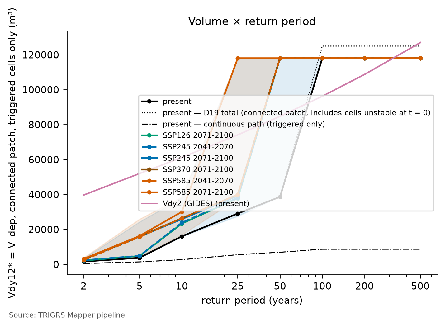
At present, V_dy12* is 29,045 m³ for TR 25, 117,992 m³ for TR 100, and 117,992 m³ for TR 200. For TR 100, the lower bound (path, triggered cells only) is 8,644 m³ and the upper bound (D19 total), 124,926 m³ — an initial share of 5.6% —, and all unstable cells add up to 156,698 m³. With the 263.7 mm of the present hyetograph, 22.5% of the watershed becomes unstable, 21.2% through triggered cells. The initial-share flag (> 10% for the present TR 100) is no: when yes, the upper bound must be read alongside V_dy12* in all tables, including in V_d*.

The curves have a plateau. Up to the present TR 50, V_dy12* grows with the rainfall; between TR 50 and TR 100 it jumps from 38,616 to 117,992 m³ and does not exceed that value up to TR 500 (Figure 8.33). The jump is one of connection, not of area: the unstable fraction of the watershed barely changes (22.2 and 22.5%), nor does the V_dep of all unstable cells (153,424 and 156,698 m³), but the few new cells connect a large, previously isolated hillslope patch to the channel. In the 88 design runs, the jump occurs between 239.9 and 247.4 mm in 24 h (Table 8.39). Above that, all the cells that the model can bring to failure are already unstable: TRIGRS limits the pressure head to that of a water table at the ground surface (Baum, Savage & Godt, 2008), and the slopes that do not fail even in that condition remain stable with any rainfall — the excess becomes runoff. Below the plateau, the curve rises in smaller steps, each one a patch that connects to the channel.

By the end of the century (P50), the TR 100 V_dy12* changes by 0.0% under SSP2-4.5 and by 0.0% under SSP5-8.5 (upper bound: 0.0% and 0.0%), whereas V_dy2 — linear in the rainfall — changes by +16.3% and +25.5% (up to +45.9% at the SSP5-8.5 P90). The present TR 100 is already on the plateau, and climate change does not change V_dy12*: the two panels of Figure 8.34 are practically identical, with the same unstable fraction (22.5 and 22.5%), although the 24-h rainfall goes from 263.7 to 330.8 mm. The same holds for TR 200 and 500 in all scenarios. TR 50 is different: at present it lies below the plateau, and almost all future scenarios reach it (see below).

Below the plateau, by contrast, V_dy12* responds to climate change much more than V_dy2. For TR 10, for example, it changes from +45.4% (SSP1-2.6) to +140.3% (SSP5-8.5 P90), against +8.6% and +36.8% for V_dy2; when the future rainfall crosses the jump, V_dy12* triples or quadruples (+205.5% for TR 50 under SSP2-4.5 P50; +306.2% for TR 25 under SSP5-8.5 P50). The 2041–2070 horizons and the SSP1-2.6 and SSP3-7.0 scenarios follow the same pattern, shifted according to the change factor; only the SSP2-4.5 P10, with a factor below 1 for some return periods, slightly reduces the volume. The upper bound does not change the reading: it follows V_dy12* below the plateau and, at the jump, grows a little more, because the cells with FS0 < 1 come to touch the large patch (+223.5% for TR 50 under SSP2-4.5 P50).

Figure 8.34: Minimum FS for TR 100 in the watershed: present vs. SSP5-8.5 2071–2100 (P50), with the 24-h rainfall and the unstable fraction of the watershed in the title of each panel.

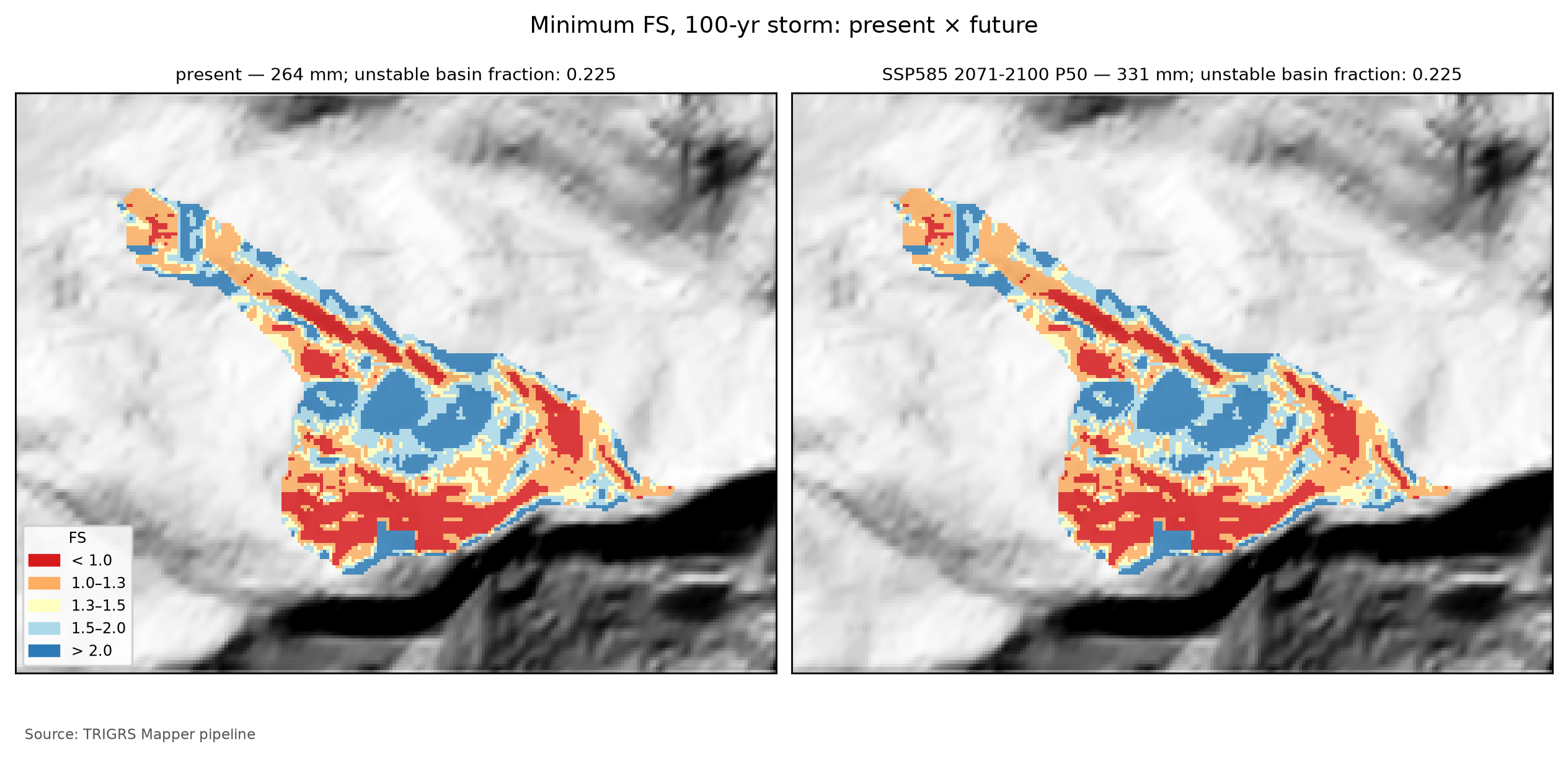
The initial condition in the watershed and land use. With the design land cover (MapBiomas 2025), 1.24% of the watershed (96 cells) has FS0 < 1 — 0 of them even without pore pressure —, against 0.17% with the event land cover (MapBiomas 2015). At t = 0, the patch of these cells is V0 = 0 m³ (all: 6,935 m³). The pipeline raises two flags, which signal without rejecting the configuration:

• FS0 < 1 in more than 1% of the watershed with the event land cover (no): a consistency warning with respect to the calibration, which required stable slopes before the event on the 30-m window;
• FS0 < 1 larger with the design land cover than with the event one (yes): a land-use effect — the slopes that lost forest between 2015 and 2025 also lost root cohesion and would be weaker today —, and not a calibration error.

When V0 is zero, the cells with FS0 < 1 do not reach the drainage on their own and only enter the upper bound if the rainfall connects them to the channel. This is what happens on the plateau: from the present TR 100 onward, the large triggered patch touches these cells, and the initial share of the total goes from zero to 5.6% — below the 10% of the flag. This is why the D19 total is still reported in all tables: excluding the initial condition must not hide an increase in hazard caused by the land-cover change.

8.10.6 From V_dy12* to V_d*: which term governs?

V_dy12* enters the manual’s accounting in place of the traditional V_dy12 (Equation 8.6):

\[ \begin{aligned} V_{dy1}^{*} &= V_{dy11} + V_{dy12}^{*}\\ V_{d}^{*} &= \max\left[\min\left(V_{dy1}^{*},\ V_{dy2}\right),\ 1{,}000\ \text{m}^3\right]\\ V_{plano}^{*} &= V_{d}^{*} + V_{w} \end{aligned} \tag{8.13}\]

with V_dy11 = 115,386 m³ (the bed; Table 8.18), the V_dy2 of each return period and scenario (Table 8.20, Table 8.21), and the woody debris V_w = 785 m³ of Section 8.7 (V_plano is the plan volume). With the upper bound of V_dy12* in place of the main value, the same calculation gives the conservative V_d*, shown in parentheses in Table 8.40. When V_dy1* < V_dy2, the volume is limited by sediment availability; when V_dy2 < V_dy1*, by the transport capacity of the rainfall — the supply-limited and transport-limited regimes of chapter 5.

Table 8.40: From TRIGRS to the design volume: Vdy12* = V_dep of the patch connected to the drainage, with the rainfall-triggered cells only (D21) → Vdy1* = Vdy11 + Vdy12* (Vdy11 = 115,386 m³) → Vd* = max(min(Vdy1*, Vdy2), 1,000 m³), against the traditional method of section 7 (Vdy12 by method b = 155,950 m³; Vdy1 = 271,336 m³). In parentheses, with D21: the upper bound of Vdy12* (D19 total, with the cells already unstable at t = 0), the Vd* recomputed with it and which term governs then, when it changes; initial share = 1 − Vdy12* ÷ total. Plan volume = Vd + woody debris (785 m³, as in section 7).

Scenario	RP (yr)	Vdy12* (upper bound) (m³)	Initial share (%)	Vdy1* (m³)	Vdy2 (m³)	Vd* (upper bound) (m³)	Governs	Trad. Vd (governs) (m³)
present	100	117,992 (124,926)	5.6	233,378	96,184	96,184 (96,184)	Vdy2	96,184 (Vdy2)
present	200	117,992 (124,926)	5.6	233,378	108,686	108,686 (108,686)	Vdy2	108,686 (Vdy2)
SSP2-4.5 2071–2100 P50	100	117,992 (124,926)	5.6	233,378	111,898	111,898 (111,898)	Vdy2	111,898 (Vdy2)
SSP2-4.5 2071–2100 P50	200	117,992 (124,926)	5.6	233,378	126,656	126,656 (126,656)	Vdy2	126,656 (Vdy2)
SSP5-8.5 2071–2100 P50	100	117,992 (124,926)	5.6	233,378	120,666	120,666 (120,666)	Vdy2	120,666 (Vdy2)
SSP5-8.5 2071–2100 P50	200	117,992 (124,926)	5.6	233,378	136,126	136,126 (136,126)	Vdy2	136,126 (Vdy2)

For the present TR 100, V_dy12* = 117,992 m³ (upper bound: 124,926 m³), against 155,950 m³ by method “b”; V_dy1* = 233,378 m³, against 271,336 m³; and V_dy2 = 96,184 m³. The sediment volume is V_d* = 96,184 m³ — the governing term is the rainfall transport capacity (Vdy2) —, or 96,184 m³ with the upper bound (governed by Vdy2); the plan volume, with woody debris, is 96,969 m³ (traditional method: V_d = 96,184 m³, governed by Vdy2).

Why V_dy2 governs at present. In Petrópolis, the bed alone already exceeds the transport capacity of the present design rainfall: V_dy11 = 115,386 m³ is larger than the V_dy2 of TR 100 (96,184 m³) and of TR 200 (108,686 m³). Since V_dy1* ≥ V_dy11 for any V_dy12*, the present-day V_d* is V_dy2, as in the traditional method (Section 8.7). Moreover, on the plateau of the curves V_dy12* alone (117,992 m³) also exceeds the V_dy2 of these return periods: for the design return periods, the conclusion does not depend on the erodible cross section adopted for the bed (20 m², without a field survey), which would only matter with a V_dy12* much smaller than the model’s.

And in the future? V_dy1* could only govern where V_dy2 > V_dy11 — for TR 500 at present and, in the future, for the highest return periods of every scenario, from TR 50 on in the wettest ones (Table 8.20, Table 8.21) —, and only if V_dy12* < V_dy2 − V_dy11. This does not happen in any of the 88 runs: when V_dy2 exceeds V_dy11, the rainfall has already brought V_dy12* to the plateau, far above the margin. Even in the extreme case, TR 500 under SSP5-8.5 P90, the margin is 192,073 − 115,386 m³, smaller than the V_dy12* of 117,992 m³. Therefore, V_dy2 governs for all return periods and scenarios, with the triggered V_dy12* and with the upper bound, and V_d* coincides with the traditional V_d: the design volume grows with climate change exactly as V_dy2 does. For TR 100 under SSP5-8.5 (P50), for example, V_dy12* = 117,992 m³ (upper bound: 124,926 m³), the governing term is Vdy2, and V_d* = 120,666 m³ (+25.5% over the present; with the upper bound, 120,666 m³). TRIGRS refines V_dy12 but does not change the design volume of Petrópolis — with or without the initial share, and with or without skill.

This result is conservative. Since the 2022 event indicates that the model overestimates the failures in Morin, a smaller actual V_dy12* could, in the scenarios with V_dy2 > V_dy11, leave V_dy1* below V_dy2 and limit the increase of the design volume by sediment availability. That reduction could only be used with a calibration that has skill and with the bed cross section measured in the field.

8.10.7 Rainfall thresholds and the Forecast tab

The thresholds answer the operational question: how much rain, in how many hours, puts the watershed at risk? The pipeline runs the watershed (30 m; D20) with uniform rainfall of increasing accumulation over durations from 1 to 72 h, for four initial water-table conditions (the working one and d = 1, 2, and 5 m), always followed by 24 h without rain, and interpolates — in the logarithm of the accumulation — the rainfall that brings 1% and 5% of the watershed to FS < 1 and the one that makes V_dy12* equal V_dy2 of the present TR 100 (96,184 m³).

With D21, the 1% and 5% fractions count only the triggered cells, and the volume criterion uses the main form of V_dy12* — here: triggered fraction of the watershed (FS0 ≥ 1 at t = 0 and FS < 1, D21); V_dy12* = V_dep of the patch connected to the drainage, with the rainfall-triggered cells only (D21). The reason is practical: with the total fraction, a watershed in which more than 1% of the cells already have FS0 < 1 would “reach” the 1% threshold with no rain at all, and the threshold would come out as “≤” because of the initial condition, not of the rainfall. This is the choice of the critical area ratio that Zhang et al. (2022) use for TRIGRS thresholds, which excludes the cells unstable without rainfall. The label of each water-table condition in Table 8.41 gives the fraction of the watershed with FS0 < 1 — with the working water table, 1.04%; with the water table at 1 m, 0.00% —, and the last two columns repeat the thresholds with the total fraction, for comparison.

Mind the resolution: for cost reasons, the Petrópolis thresholds use the 30-m watershed (D20), not the 10-m one of the design runs. The area criteria (1% and 5% of the watershed) do not depend on the connection to the drainage, but the volume criterion does: at 30 m the patch connected to the channel is larger than at 10 m (Section 8.10.2), and V_dy12* reaches V_dy2 with a little less rain. In 24 h, the volume threshold at 30 m is 235 mm; in the design curves of the 10-m watershed, with differently shaped hyetographs, V_dy12* exceeds V_dy2 between 239.9 and 247.4 mm. Read the volume threshold as slightly conservative.

Table 8.41: Physical thresholds of uniform rainfall (accumulated over D hours) that bring 1% and 5% of the watershed to FS < 1 and the Vdy12* up to the present 100-yr Vdy2 (96,184 m³). 1% and 5% counted with the triggered fraction of the watershed (FS0 ≥ 1 at t = 0 and FS < 1, D21). Vdy12*: V_dep of the patch connected to the drainage, with the rainfall-triggered cells only (D21). Watershed at 30 m, calibrated configuration, 24-h post-rain window. “≤” = already reached at the smallest accumulation tested (10 mm); “>” = not reached up to 540 mm. With the triggered fraction, the instability that already exists without rain (FS0 < 1, shown for each water table) does not “reach” the threshold; the last two columns repeat the thresholds with the total fraction, for comparison.

Initial water table	Duration (h)	1% of the watershed — triggered (mm)	5% of the watershed — triggered (mm)	Vdy12* ≥ Vdy2 (mm)	1% — total fraction (mm)	5% — total fraction (mm)
base (0.50·zmax) — FS0 < 1: 1.04%	1	14	46	106	≤ 10	40
base (0.50·zmax) — FS0 < 1: 1.04%	3	28	65	113	≤ 10	59
base (0.50·zmax) — FS0 < 1: 1.04%	6	46	84	134	≤ 10	78
base (0.50·zmax) — FS0 < 1: 1.04%	12	80	110	167	≤ 10	101
base (0.50·zmax) — FS0 < 1: 1.04%	24	134	182	235	≤ 10	174
base (0.50·zmax) — FS0 < 1: 1.04%	48	261	282	316	≤ 10	276
base (0.50·zmax) — FS0 < 1: 1.04%	72	334	367	428	≤ 10	358
d = 1 m — FS0 < 1: 0.00%	1	54	160	> 540	54	160
d = 1 m — FS0 < 1: 0.00%	3	76	160	208	76	160
d = 1 m — FS0 < 1: 0.00%	6	95	173	221	95	173
d = 1 m — FS0 < 1: 0.00%	12	142	208	238	142	208
d = 1 m — FS0 < 1: 0.00%	24	224	276	311	224	276
d = 1 m — FS0 < 1: 0.00%	48	332	358	400	332	358
d = 1 m — FS0 < 1: 0.00%	72	425	461	524	425	461
d = 2 m — FS0 < 1: 0.00%	1	54	174	> 540	54	174
d = 2 m — FS0 < 1: 0.00%	3	76	177	265	76	177
d = 2 m — FS0 < 1: 0.00%	6	101	206	307	101	206
d = 2 m — FS0 < 1: 0.00%	12	162	242	321	162	242
d = 2 m — FS0 < 1: 0.00%	24	229	335	442	229	335
d = 2 m — FS0 < 1: 0.00%	48	387	477	> 540	387	477
d = 2 m — FS0 < 1: 0.00%	72	518	> 540	> 540	518	> 540
d = 5 m — FS0 < 1: 0.00%	1	54	174	> 540	54	174
d = 5 m — FS0 < 1: 0.00%	3	76	177	265	76	177
d = 5 m — FS0 < 1: 0.00%	6	101	206	307	101	206
d = 5 m — FS0 < 1: 0.00%	12	162	242	321	162	242
d = 5 m — FS0 < 1: 0.00%	24	229	335	442	229	335
d = 5 m — FS0 < 1: 0.00%	48	387	477	> 540	387	477
d = 5 m — FS0 < 1: 0.00%	72	518	> 540	> 540	518	> 540

With the working water table (0.50·zmax), 24-h rainfalls bring 1% of the watershed to FS < 1 with 134 mm, 5% with 182 mm, and V_dy12* up to V_dy2 with 235 mm; in 6 h, the thresholds are 46, 84, and 134 mm; in 72 h, 334, 367, and 428 mm. With the water table at 1 m, the 24-h threshold for 5% of the watershed is 276 mm. The prefix “≤” means that the criterion is already met at the smallest accumulation tested, and “>”, that it was not met up to 540 mm.

Triggered fraction vs. total fraction. By the triggered fraction, no threshold comes out as “≤”, but the short-duration ones lie close to the smallest accumulation tested — 14 mm in 1 h bring 1% of the watershed to failure —: with the working water table, a wet, storm-like state, part of the slopes is already close to failure before the rain. By the total fraction, the 1% threshold comes out as “≤ 10” mm for every duration, because 1.04% of the 30-m watershed already has FS0 < 1 with this water table: this is exactly the effect that D21 removes. With the water table at 1 m or deeper, no cell has FS0 < 1, and both fractions give the same thresholds.

Thresholds vs. design rainfall and the 2022 rainfall. By the 24-h total — the design hyetographs concentrate the rainfall, whereas the thresholds spread it uniformly —, 1% of the watershed fails with a rainfall between those of TR 2 and TR 5 (108.6 and 142.5 mm), 5% with a rainfall between those of TR 10 and TR 25 (167.7 and 203.0 mm), and V_dy12* reaches V_dy2 at about the TR 50 rainfall (232.1 mm), below the TR 100 one (263.7 mm). The February 15, 2022 storm exceeds all the 3-h and 6-h thresholds by a wide margin: almost all of the 223 mm of the central scenario fell in 3 h (Table 8.14), and even the minimum scenario (Bingen, 142 mm) exceeds the three criteria for these durations. According to the model, the Morin watershed would have failed on a large scale in 2022 — which did not happen (Section 8.9). The Petrópolis thresholds therefore inherit the lack of skill of the configuration: they hold as a scenario, tend to be too low, and must not guide warnings before a new calibration.

These thresholds feed the Forecast (Previsão) tab of the TRIGRS Mapper portal (planned domain trigrs.dpm-sedec-sas.tech, being deployed), which has three modes: (i) scenario — the user sets the rainfall (accumulation, duration, and pattern, or a hyetograph), the antecedent rainfall, the initial water table, and the multipliers, and TRIGRS runs on demand on the 10-m watershed; (ii) physical thresholds — the curves of Table 8.41, to compare with the observed or forecast rainfall; (iii) experimental numerical forecast — hourly rainfall from the ECMWF IFS, GFS, and ICON models (Open-Meteo service) for the next 72 h, one run per model. The runs of the tab use the 10-m watershed, and the result is classified, like the thresholds, by the triggered fraction (D21): green (< 1% of the watershed with FS < 1 through triggered cells), yellow (≥ 1%), orange (≥ 5%), and red (V_dy12* ≥ V_dy2). The cells already unstable without rain are shown separately, without changing the class.

WarningExperimental tool

The Forecast tab is a research prototype: it uses parameters calibrated with preliminary scars — in Petrópolis, subject to the skill flag of Section 8.9 —, rainfall forecast by global models with a resolution of tens of kilometers, and an infinite-slope model without propagation of the failed mass. It does not replace the official warnings of Cemaden and the Civil Defense nor the municipal contingency plans.

8.11 Synthesis, limitations and recommendations

Table 8.42 gathers the main numbers of the TRIGRS × GIDES coupling in Petrópolis.

Table 8.42: Summary of the TRIGRS × GIDES results for Petrópolis. Vdy12* = V_dep of the patch connected to the drainage, with the rainfall-triggered cells only (D21); the D19 total (with the cells already unstable at t = 0) is the upper bound.

Quantity	Value	Note
Watershed area (km²)	0.771	7,712 cells of 10 m
Calibration — triggered MSR / MSR / AUC of the best sample	0.52 / 0.53 / 0.58	selected by triggered MSR; a priori: 0.49 / 0.49 / 0.57; 150 LHS samples in the 30 m window
Calibration — feasible samples (D21 filters) and relaxed constraints	18 of 150	relaxed: median Z_cr, unstable area and AUC
Calibration — triggered TSS / AUC (skill)	0.04 / 0.58	no skill: yes (triggered TSS < 0.05 or AUC < 0.60)
Cross-validation — transferred MSR	0.54 — Cuiabá Valley, Jan 2011 (D16)	a priori at the target: 0.52
Event — unstable fraction of the watershed (%)	22.1	17.06 ha unstable
Event — Vdy12* (m³)	121,626	D19 total (upper bound): 122,635; all: 154,407; in situ (all): 170,167
Initial condition — FS0 < 1 in the watershed: design / event (%)	1.24 / 0.17	patch Vdep at t = 0 (design): 0 m³; FS0 < 1 with the event land cover: 0.17%
Vdy12 — traditional (method b) × Vdy12* (100-yr, present; m³)	155,950 × 117,992	D19 total (upper bound): 124,926; initial share: 5.6%
Vdy1 — traditional × Vdy1* (100-yr, present; m³)	271,336 × 233,378
Vdy2 — 100-yr: present / SSP2-4.5 / SSP5-8.5 2071–2100 P50 (m³)	96,184 / 111,898 / 120,666
Vd — traditional × Vd* (100-yr, present; m³)	96,184 (Vdy2) × 96,184 (Vdy2)	Vd* with the upper bound: 96,184; woody debris: Vwy = 785 m³
Vd* — 100-yr: SSP2-4.5 / SSP5-8.5 2071–2100 P50 (m³)	111,898 (Vdy2) / 120,666 (Vdy2)
Vdy12* — change SSP5-8.5 2071–2100 P50 vs. present, 100-yr (%)	0.0	D19 total: 0.0%
24-h threshold, base water table — 1% / 5% of the watershed / Vdy12* ≥ Vdy2 (mm)	134 / 182 / 235	watershed at 30 m; triggered fraction of the watershed (FS0 ≥ 1 at t = 0 and FS < 1, D21)
Most influential factor on the event Vdep	flowdir = hydro (+103.0 %)
Resolution — patch Vdep at 10 m × 30 m (%)	−32.8
State of the results	final — full

8.11.1 What the Petrópolis case teaches

1. The design watershed is not the laboratory. In 2022 the scars were concentrated in Alto da Serra and Morro da Oficina, 1.2–1.6 km from the reference point, and the Morin watershed hardly failed. The calibration used the Alto da Serra scars, and the watershed itself became a specificity test, which showed the model overestimating the failures there (Section 8.9).
2. The timing of the failure matters. TRIGRS starts from an initial condition that can leave slopes unstable before any rain, and calibrating by the total MSR rewarded those slopes: in Petrópolis, the sample with the highest total MSR has most of the event’s unstable cells already unstable before it. With D21, the selection uses the triggered MSR with filters of stability before the event, and the volumes count only what the rainfall triggers: the initial condition is kept apart, as an upper bound and as V0 — here, with a small weight (initial share of 5.6% for TR 100).
3. No skill in Petrópolis, and a validation only counts if it is independent. The best sample has triggered TSS = 0.04 and AUC = 0.58 against the 2022 scar candidates (flag sem_habilidade: yes). Transferred to the Vale do Cuiabá, it outperforms the a priori run and meets the D21 minimums (triggered MSR 0.54; AUC 0.72), but that window covers 66.5% of the calibration window and 96.2% of the watershed of Teresópolis and uses the 2011 Teresópolis rainfall: it says little about Petrópolis and nothing about the 2022 rainfall. With that rainfall, the model puts 22.1% of the Morin watershed, which hardly failed, at FS < 1: it overestimates the instability, and the lack of skill cannot be attributed to the preliminary inventory alone. The TRIGRS volumes hold as a scenario of a stable configuration, not as a calibrated prediction; the recalibration with the municipal inventory is the next step, with no guarantee that it will be enough.
4. V_dy2 always governs. V_dy11 alone exceeds the V_dy2 of the present TR 100 and 200, and, when V_dy2 exceeds V_dy11 (rare return periods and future climate), V_dy12* is already on the plateau: in none of the 88 runs does V_dy1* govern. TRIGRS replaces the method “b” V_dy12 (155,950 m³) with a physical value (117,992 m³ for TR 100; upper bound: 124,926 m³), but does not change the design volume.
5. Form and connection weigh as much as the physics. The same TRIGRS result ranges from 8,644 m³ (path V_dep, triggered cells only) to 283,612 m³ (V_solto of all unstable cells) for the event (Table 8.38), the fraction connected to the channel depends on the resolution, and the plateau of the curves arises from a jump in connection, not in area. Stating the form, the connectivity, and whether the initial condition is included is part of the result.
6. Climate. V_dy2 grows in proportion to the daily rainfall (+25.5% for TR 100 under SSP5-8.5, end of the century). V_dy12* responds in steps: below the plateau, much more than the rainfall; on the plateau — where the present TR 100 already lies —, not at all (0.0%; upper bound: 0.0%). In Petrópolis, the whole effect of climate change on the design volume goes through V_dy2.
7. TRIGRS adds the when and the how much, not the where. Slope alone ranks the source areas as well as the calibrated FS (AUC 0.58 vs. 0.58; better in Nova Friburgo and in Teresópolis), and the failure depth is the thickness of the zmax model (Z_cr = zmax in 100.0% of the unstable cells of the event). What the coupling adds to the GIDES method is the triggering over time — which rainfall brings the hillslopes to failure, in the thresholds and in the future climate — and the count of the volume connected to the drainage; the thickness, which sets that volume, needs field measurements.

8.11.2 Implications for the Sabo dam

• Design volume. For the present TR 100, the plan volume is 96,969 m³ (V_d* + woody debris), the same as with the traditional method: V_dy2 governs for all return periods and scenarios, with the triggered V_dy12* and with the upper bound (Section 8.10). The reference point lies 72 m upstream of the first houses, with no free deposition reach between the valley and the built-up area (Section 8.2): the structure must retain the entire design volume.
• Climate. Since V_dy2 governs and is linear in the rainfall, the TR 100 design volume grows by +16.3% (SSP2-4.5) and +25.5% (SSP5-8.5) by the end of the century (P50), and today’s 100-year rainfall becomes a 20- to 60-year event (Table 8.16). A design with a climate margin should consider at least the P50 of these scenarios.
• Scenario, not calibration. TRIGRS does not reduce the design volume in any scenario, and therefore the skill flag does not change V_d*. But the Petrópolis V_dy12* is a scenario and, judging by the 2022 event, probably overestimated: with a calibration that has skill, a smaller V_dy12* could, for rare return periods and in the future climate, limit the volume by sediment availability. Until then, the conservative references are V_dy2 and the V_d* with the upper bound of V_dy12*.
• Thresholds. According to the model, frequent rainfalls already bring part of the watershed to failure, and the 2022 storm would have brought it to failure on a large scale (Section 8.10). Since the watershed hardly failed, the Petrópolis thresholds are too low for warnings until the recalibration.
• Peak discharge. Q_sp depends on V_d and, above all, on the empirical coefficient (0.002 of the manual vs. 0.01 of the Japanese standard; Section 8.7.6) — a discrepancy to be resolved before the hydraulic design.
• Bed survey. The erodible cross section of the bed (B_d·D_e) sets V_dy11, which with the adopted section is enough for V_dy2 to govern at present; with a calibrated V_dy12* smaller than the model’s, it would decide whether the design volume can fall below V_dy2. It is the first field data to obtain.

8.11.3 Uncertainties and limitations

1. Event rainfall constructed from published values (D14), uniform over the window and without an observed hourly series; the rainfall over the watershed is unknown, and the sensitivity to the event scaling has not been run.
2. Inventory: preliminary, unvalidated Sentinel-2 candidates; source area approximated by the upper third; urban fabric excluded; scars smaller than a 30-m cell poorly resolved. It is a likely cause of the lack of skill, but not the only one: with the 2022 rainfall, the model puts 22.1% of the Morin watershed at FS < 1, where there are almost no scars, and neither the Vale do Cuiabá validation (overlapping the Teresópolis area) nor the window re-evaluated at 10 m (with fewer unstable cells) isolates the effect of the inventory.
3. Parameters a priori from the literature, without laboratory tests in Petrópolis; θ_s and G_s fixed; the same values for all lithologies.
4. Soil thickness from slope only, with the 1-m cap inherited from a 1:250,000 soil unit (AR3), a scale that does not resolve the hillslope; no measurements. Since Z_cr = zmax in 100.0% of the unstable cells, V_dy12* inherits this model directly, and the calibration on the window hardly constrains it.
5. Initial water table without measurements: f_NA is an effective parameter (the moisture left by previous rains), kept the same at present and in the future, and the volumes hold for this initial condition; the D6 scenarios give the sensitivity.
6. Initial condition and land use: the 10-m watershed with the 2025 land cover may have cells with FS0 < 1 that the 30-m window, with the 2015 one, did not show; they stay out of V_dy12* and enter the upper bound.
7. Selection: the gaps between the top samples are small, but they draw very different maps, and the limits of the filters (1%, 5%, 30%, and 0.05) come from the literature, not from local data.
8. Resolution: 10-m DEM resampled from the 30-m ANADEM; the connection to the drainage depends on the resolution, and the plateau of the curves arises from the connection of a single large patch to the channel. The parameters were calibrated at 30 m and applied at 10 m, and they are not independent of resolution: on the window, the same set makes 14.8% of the cells unstable at 10 m, against 20.6% at 30 m.
9. Model: one-dimensional infinite slope, without lateral subsurface flow or propagation of the mass; the connection to the drainage is an indicator, not a simulation of the flow.
10. Design runs: the same antecedent condition (the rizero and f_NA calibrated for February 2022) for all return periods and scenarios.
11. Climate: only the daily rainfall changes; sub-daily rainfall and multi-day accumulations are not in the factors (Section 8.6).
12. Validation: a single cross-validation (Vale do Cuiabá, 2011, with the reconstructed Teresópolis rainfall), and it is not independent: the window covers 66.5% of the calibration window and 96.2% of the watershed of Teresópolis. There is no validation of the configuration in Petrópolis with another rainfall: the March 20, 2022 event has not been run.
13. Spatial ranking: with the same positives and negatives, slope alone ranks the source areas as well as the calibrated FS (AUC 0.58 vs. 0.58; in Nova Friburgo, 0.70 vs. 0.66, and in Teresópolis, 0.85 vs. 0.76). The FS map does not rank the hillslopes better than slope, and the use of TRIGRS in this chapter rests on the triggering over time and on the volume.

8.11.4 Recommendations

1. 2022 municipal inventory: request from the Petrópolis City Hall and Civil Defense the inventory with failure and deposit mapped separately (> 370 landslides; Ochi et al., 2022) and the polygons of Alcântara et al. (2023), and redo the calibration with them — the priority step, because it separates what comes from the reference from what comes from the model. It does not guarantee skill: if the model keeps bringing a large part of the watershed to failure without scars, the cause lies in the parameters, the thickness, or the rainfall (recommendations 2 to 5).
2. Rainfall: obtain the hourly series from Cemaden (São Sebastião, Dr. Thouzet, Morin) and INEA (Alto da Serra) and run the sensitivity to the event scaling (minimum and maximum scenarios).
3. Geotechnical tests in the shallow soils, colluvia, and residual soil of the watershed: c′, φ′, K_s, and the retention curve (θ_s, θ_r, and α) on undisturbed samples, to replace the a priori values.
4. Measured water table: piezometers and tensiometers on representative slopes for at least one rainy season, to pin down the initial water table and the background infiltration and replace the effective f_NA with an observed value.
5. LiDAR and field survey: soil thickness (boreholes, trenches, depth of the scars) — since Z_cr = zmax, it is the data that directly sets V_dy12* —, bed cross sections (B_d and D_e of V_dy11), and a high-resolution DEM, which reduces the dependence of the connection to the drainage on the resolution.
6. Independent validation: separate the March scars (Sentinel-2 pair March 4 × April 23, 2022) and run the March 20, 2022 event with the calibrated configuration, the first validation in Petrópolis with another rainfall. In a new cross-validation, use a window with no overlap with the calibration windows and watersheds of the other cases.
7. Regional configuration: as a sensitivity case, run the Petrópolis design with sample lhs_0019, the one chosen in Nova Friburgo and in Teresópolis — the LHS design is the same in the three cases; in Petrópolis it passes the filters, with a smaller unstable area than the winner —, and compare the volumes.
8. Forecast: compare the thresholds and the runs of the Forecast tab with the rainfall and landslides of the next rainy seasons before any operational use.

8.12 Reproducibility

Everything shown in sections 8.8 to 8.11 can be reproduced from the root of the trigrs-mapper project (the companion), with the Python 3.12 of the project environment and TRIGRS 2.1 compiled in engine/bin. The commands of each step, the time of each one, and the versions are below (Table 8.43, Table 8.44).

Reproducing the case (at the root of the trigrs-mapper project)

# everything, in order (the event runs before and after the calibration)
scripts/pipeline/rodar_caso.sh petropolis --max-cpus 8 --mpi
# or stage by stage
.venv/bin/trigrs-mapper caso petropolis grades
.venv/bin/trigrs-mapper caso petropolis calibrar --max-cpus 8      # LHS + cross-validation
.venv/bin/trigrs-mapper caso petropolis params
.venv/bin/trigrs-mapper caso petropolis evento --max-cpus 8 --mpi
.venv/bin/trigrs-mapper caso petropolis projeto --max-cpus 8
.venv/bin/trigrs-mapper caso petropolis sensibilidade --max-cpus 8 --mpi
.venv/bin/trigrs-mapper caso petropolis limiares --max-cpus 8
.venv/bin/trigrs-mapper caso petropolis produtos
.venv/bin/trigrs-mapper caso petropolis figuras
# numbers, tables and figures of these sections (PT and EN)
.venv/bin/python scripts/capitulos/gerar_resultados_trigrs.py --destino <short-course repository>

Table 8.43: Pipeline stages of this case (command trigrs-mapper caso <case> <stage>; manifests data/cases/<case>/logs/etapa_*.json): mode, CPUs, wall-clock duration and, for stages with serial runs, the sum of the TRIGRS run durations (CPU·h). Shared 12-core VPS; times vary with the load.

Stage	Command	Mode; status	CPUs	Duration (h)	CPU·h (runs)	End (Brasília)
grids	grades	full; completed	2	< 0.01	n/a	2026-10-31 18:48
calibration + cross-validation	calibrar	full; completed	2	0.11	9.7	2026-11-01 00:10
parameterization (documentation)	params	full; completed	3	< 0.01	n/a	2026-11-01 00:10
event (30 m window + 10 m watershed)	evento --mpi	full; completed	3	0.06	n/a	2026-11-01 00:14
design runs (return period × scenarios)	projeto	full; completed	3	0.45	1.3	2026-11-01 00:41
sensitivity	sensibilidade --mpi	full; completed	3	0.52	1.0	2026-11-01 01:13
thresholds	limiares	full; completed	3	0.14	n/a	2026-11-01 01:21
products	produtos	full; completed	1	< 0.01	n/a	2026-11-01 03:51
figures	figuras	full; completed	1	< 0.01	n/a	2026-11-01 02:23

Table 8.44: Environment versions recorded in the stage manifests (run completed on 2026-11-01).

Component	Version / identification
TRIGRS (serial)	2.1.00a (26 Aug 2016); SHA-256 afb53a06daa4…
TopoIndex	SHA-256 832f46b4023a…
TRIGRS-P (MPI)	SHA-256 5b20f00464c9…
Python	3.12.15
gdal	3.12.2
geopandas	1.2.0
matplotlib	3.11.2
numpy	2.5.4
pandas	3.1.0
pyproj	3.8.0
rasterio	1.5.2
scipy	1.18.1
shapely	2.2.0
trigrs-mapper	0.1.0
Platform	Linux-5.15.0-198-generic-x86_64-with-glibc2.35

The full run of this case uses the driver of decision D20, which runs the steps in order with low priority and waits for a manual release after the calibration. With D21, the selection is redone before the release, with the objective and the filters of the case YAML, reusing the runs already made:

Full run (D20 and D21), at the root of the trigrs-mapper project

# grades → calibrar (+ cross-validation) → [D21 selection and release] → params → evento → projeto
#   → produtos → figuras → sensibilidade → limiares → produtos → figuras
nohup scripts/pipeline/rodar_completo.sh petropolis 2 > /dev/null 2>&1 &
# D21: redoes the selection (triggered MSR + filters of configs/cases/petropolis.yaml) and the
# cross-validation; the 151 calibration runs are reused through their signatures
nice -n 10 .venv/bin/trigrs-mapper caso petropolis calibrar --forcar --max-cpus 2
touch _operacional/rodada_completa/liberar_petropolis    # releases the steps after checking the calibration
.venv/bin/trigrs-mapper estado petropolis                 # status of the steps
# smoke test (6 LHS samples; 2 TR × 2 scenarios; reduced sensitivity and thresholds)
scripts/pipeline/rodar_caso.sh petropolis --reduzido --max-cpus 8
# independent diagnostics (slope AUC, Z_cr = zmax, resolution, Vale do Cuiabá overlap)
.venv/bin/python scripts/capitulos/diagnosticos_independentes.py petropolis
# numbers, tables, and figures of the TRIGRS sections (PT and EN); idempotent
.venv/bin/python scripts/capitulos/gerar_resultados_trigrs.py --casos petropolis
.venv/bin/python scripts/capitulos/gerar_resultados_trigrs.py --verificar   # writes nothing; exit code 1 if anything would change

Versions and run times. TRIGRS 2.1.00a (26 Aug 2016; SHA-256 afb53a06daa4…), Python 3.12.15, numpy 2.5.4, scipy 1.18.1, rasterio 1.5.2, and GDAL 3.12.2. The 151 calibration runs (full) add up to 9.7 CPU·h; the last pass of the step — the D21 calibrar --forcar, which only redid the selection and the cross-validation, reusing the runs — took 0.11 h of wall-clock time with 2 CPUs. The event took 0.06 h; the design runs, 0.45 h (1.3 CPU·h); the sensitivity analysis, 0.52 h (1.0 CPU·h of runs); the thresholds, 0.14 h — in all, 1.29 h for the last passes of the steps (the last one on 2026-11-01), on a shared 12-core VPS.

Where the data are (outside the short-course repository; recreated by the commands above and checked by the SHA-256 checksums of the manifests):

• inputs, read-only: data/cases/petropolis/{bacia,chuva,gides} (sections 8.1 to 8.7), data/interim/{bases,parametros,clima}, the images and the inventory in data/raw/, and ANADEM;
• case configuration: configs/cases/petropolis.yaml (objective and filters of the selection, main form of V_dy12*, and initial condition — decisions D20 and D21);
• grids and parameterization: data/cases/petropolis/grids/<domain>_<res>m/, with params_<land cover>/ (zones, zmax, depthwt, rizero, units);
• runs: data/cases/petropolis/runs/ (tr_in.txt, tpx_in.txt, rodada.json, resultado.json — with the signature and the fraction of non-converged cells — and resultado.npz with FS and Z_cr of each output);
• calibration, event, design, and sensitivity: data/cases/petropolis/calibracao/ (calibracao.json, with the record of the selection — stages, exclusion reasons, and warnings —, lhs.csv, melhor.json, with the objective, the filters, and the skill flag, conjunto/, validacao_cruzada.json, evento/, projeto.json, projeto_condicao_inicial.npz, with the FS0 and Z_cr of t = 0, sensibilidade.json, and diagnosticos.json, with the independent diagnostics of sections 8.9 and 8.10);
• portal products: data/cases/petropolis/produtos/ (resumo.json, COG layers, GeoJSON vectors, series, animation, and figures) and data/produtos/casos.json;
• manifests and logs: data/cases/petropolis/logs/etapa_<step>.json (arguments, signature, versions, SHA-256 of the executables, duration) and the logs of each step.

Each step is idempotent: with the same signature (arguments, case YAML, parameter table, calibration in use, and rainfall and GIDES files) it is skipped; --forcar redoes it, reusing identical runs. FS0 requires no run: trigrs_mapper.trigrs.fs_inicial computes it in closed form, with a test against the executable (tests/test_fs_inicial.py). Rendering the book does not run TRIGRS: the numbers come from the generator, checked by automated tests (tests/test_gerar_resultados.py).

References cited in this chapter

• Alcântara, E. et al. (2023). Deadly disasters in southeastern South America: flash floods and landslides of February 2022 in Petrópolis, Rio de Janeiro. Natural Hazards and Earth System Sciences, 23, 1157–1175. doi:10.5194/nhess-23-1157-2023
• Anderson, R. L. (1942). Distribution of the serial correlation coefficient. Annals of Mathematical Statistics, 13(1), 1–13.
• Barnes, R.; Lehman, C.; Mulla, D. (2014). An efficient assignment of drainage direction over flat surfaces in raster digital elevation models. Computers & Geosciences, 62, 128–135. doi:10.1016/j.cageo.2013.01.009
• Baum, R. L.; Godt, J. W.; Savage, W. Z. (2010). Estimating the timing and location of shallow rainfall-induced landslides using a model for transient, unsaturated infiltration. Journal of Geophysical Research: Earth Surface, 115, F03013. doi:10.1029/2009JF001321
• Baum, R. L.; Savage, W. Z.; Godt, J. W. (2008). TRIGRS — A Fortran program for transient rainfall infiltration and grid-based regional slope-stability analysis, version 2.0. U.S. Geological Survey Open-File Report 2008-1159. doi:10.3133/ofr20081159
• Blaudt, Alvarenga & Garin (2023). Geociências (UNESP) — hourly maximum at São Sebastião on February 15, 2022 (cited in docs/pesquisa/02_inventarios.md).
• Brasil. Ministério da Integração Nacional [Ministry of National Integration]; JICA (2018, rev. 2019). Manual técnico para concepção de intervenções para fluxo de detritos [Technical manual for the design of debris-flow interventions] (GIDES Project), §2.4–2.5, Annexes 1–4 and Appendix A. In Portuguese.
• Cemaden (2022). Nota técnica: desastres ocorridos na cidade de Petrópolis, RJ — eventos de 15/02/2022 e 20/03/2022 [Technical note: disasters in the city of Petrópolis, RJ — events of February 15 and March 20, 2022]. Attached to Ofício nº 5111/2022/MCTI [official letter] (Federal Senate). In Portuguese.
• Chow, V. T. (1962). Hydrologic determination of waterway areas for the design of drainage structures in small drainage basins. Univ. of Illinois, Engineering Experiment Station, Bulletin 462.
• Chow, V. T.; Maidment, D. R.; Mays, L. W. (1988). Applied Hydrology. McGraw-Hill.
• Coelho Netto, A. L. et al. (2022). The most recent disaster related to extreme rainfall induced landslides and floods: Petropolis, Rio de Janeiro state, SE-Brazil. 10th International Conference on Geomorphology, Coimbra, ICG2022-628. doi:10.5194/icg2022-628
• Cohen, J. (1960). A coefficient of agreement for nominal scales. Educational and Psychological Measurement, 20(1), 37–46. doi:10.1177/001316446002000104
• Custódio, M. R. C. et al. (2023). Mapeamento da distribuição pluviométrica e das áreas afetadas no desastre de Petrópolis em fevereiro de 2022 [Mapping of the rainfall distribution and of the affected areas in the February 2022 Petrópolis disaster]. VI Congresso Internacional de Riscos, Coimbra (abstract). In Portuguese.
• DAEE/CETESB (1980). Drenagem urbana: manual de projeto [Urban drainage: design manual]. São Paulo: DAEE/CETESB. In Portuguese.
• DeRose, R. C. (1996). Relationships between slope morphology, regolith depth, and the incidence of shallow landslides in eastern Taranaki hill country. Zeitschrift für Geomorphologie, Supplementband 105, 49–60.
• Emberson, R.; Kirschbaum, D. B.; Amatya, P.; Tanyas, H.; Marc, O. (2022). Insights from the topographic characteristics of a large global catalog of rainfall-induced landslide event inventories. Natural Hazards and Earth System Sciences, 22, 1129–1149. doi:10.5194/nhess-22-1129-2022
• Fawcett, T. (2006). An introduction to ROC analysis. Pattern Recognition Letters, 27(8), 861–874. doi:10.1016/j.patrec.2005.10.010
• Formetta, G.; Capparelli, G.; Versace, P. (2016). Evaluating performance of simplified physically based models for shallow landslide susceptibility. Hydrology and Earth System Sciences, 20, 4585–4603. doi:10.5194/hess-20-4585-2016
• Gardner, W. R. (1958). Some steady-state solutions of the unsaturated moisture flow equation with application to evaporation from a water table. Soil Science, 85(4), 228–232.
• Giandotti, M. (1934). Previsione delle piene e delle magre dei corsi d’acqua. Memorie e Studi Idrografici, 8.
• Gringorten, I. I. (1963). A plotting rule for extreme probability paper. Journal of Geophysical Research, 68(3), 813–814. doi:10.1029/JZ068i003p00813
• Hershfield, D. M. (1961). Rainfall frequency atlas of the United States for durations from 30 minutes to 24 hours and return periods from 1 to 100 years. Technical Paper No. 40. Washington, DC: U.S. Weather Bureau.
• Horn, B. K. P. (1981). Hill shading and the reflectance map. Proceedings of the IEEE, 69(1), 14–47. doi:10.1109/PROC.1981.11918
• Hosking, J. R. M.; Wallis, J. R. (1997). Regional Frequency Analysis: an approach based on L-moments. Cambridge University Press. doi:10.1017/CBO9780511529443
• Huang, J. C.; Kao, S. J. (2006). Optimal estimator for assessing landslide model performance. Hydrology and Earth System Sciences, 10, 957–965. doi:10.5194/hess-10-957-2006
• IACWD (1982). Guidelines for determining flood flow frequency — Bulletin 17B. U.S. Interagency Advisory Committee on Water Data.
• José, F. O. (2016). Análise do incremento de resistência ao cisalhamento do solo conferido por raízes florestais em Nova Friburgo, RJ [Analysis of the increase in soil shear strength provided by forest roots in Nova Friburgo, RJ]. M.Sc. dissertation (Civil Engineering) — COPPE/UFRJ. In Portuguese.
• Kirpich, Z. P. (1940). Time of concentration of small agricultural watersheds. Civil Engineering, 10(6), 362.
• Laipelt, L. et al. (2024). ANADEM: A Digital Terrain Model for South America. Remote Sensing, 16(13), 2321. doi:10.3390/rs16132321
• Marc, O.; Stumpf, A.; Malet, J.-P.; Gosset, M.; Uchida, T.; Chiang, S.-H. (2018). Initial insights from a global database of rainfall-induced landslide inventories: the weak influence of slope and strong influence of total storm rainfall. Earth Surface Dynamics, 6, 903–922. doi:10.5194/esurf-6-903-2018
• Massad, F. et al. (1997), cited in the SABO Manual Vol. 1 (SEDEC/MIDR and JICA, 2026), Eq. 22 (I₁ ≈ 0.28·Pp).
• McKay, M. D.; Beckman, R. J.; Conover, W. J. (1979). A comparison of three methods for selecting values of input variables in the analysis of output from a computer code. Technometrics, 21(2), 239–245.
• NILIM (2016). Manual of technical standard for establishing Sabo master plan for debris flow and driftwood. Technical Note of NILIM No. 904. Tsukuba.
• O’Callaghan, J. F.; Mark, D. M. (1984). The extraction of drainage networks from digital elevation data. Computer Vision, Graphics, and Image Processing, 28(3), 323–344.
• Ochi, H.; Shimoda, Y.; Nishio, Y.; Machado, R. P. (2022). Sediment-related disasters in Petrópolis, Brazil, on February 15 and March 20, 2022. International Journal of Erosion Control Engineering, 15(3), 31–38. doi:10.13101/ijece.15.31
• Papalexiou, S. M.; Koutsoyiannis, D. (2013). Battle of extreme value distributions: a global survey on extreme daily rainfall. Water Resources Research, 49(1), 187–201. doi:10.1029/2012WR012557
• Park, D. W.; Nikhil, N. V.; Lee, S. R. (2013). Landslide and debris flow susceptibility zonation using TRIGRS for the 2011 Seoul landslide event. Natural Hazards and Earth System Sciences, 13, 2833–2849. doi:10.5194/nhess-13-2833-2013
• Pinho et al. (2013), cited in Appendix A of the GIDES manual (Table 3.1: scar density by slope class in Córrego D’Antas).
• Poggio, L. et al. (2021). SoilGrids 2.0: producing soil information for the globe with quantified spatial uncertainty. SOIL, 7, 217–240. doi:10.5194/soil-7-217-2021
• Potapov, P. et al. (2022). The global 2000–2020 land cover and land use change dataset derived from the Landsat archive. Remote Sensing, 14(16), 4101. doi:10.3390/rs14164101
• Raia, S.; Alvioli, M.; Rossi, M.; Baum, R. L.; Godt, J. W.; Guzzetti, F. (2014). Improving predictive power of physically based rainfall-induced shallow landslide models: a probabilistic approach. Geoscientific Model Development, 7, 495–514. doi:10.5194/gmd-7-495-2014
• Salciarini, D.; Godt, J. W.; Savage, W. Z.; Conversini, P.; Baum, R. L.; Michael, J. A. (2006). Modeling regional initiation of rainfall-induced shallow landslides in the eastern Umbria Region of central Italy. Landslides, 3(3), 181–194. doi:10.1007/s10346-006-0037-0
• Sartori, A.; Lombardi Neto, F.; Genovez, A. M. (2005). Classificação hidrológica de solos brasileiros para a estimativa da chuva excedente com o método do Serviço de Conservação do Solo dos Estados Unidos. Parte 1: classificação [Hydrologic classification of Brazilian soils for estimating excess rainfall with the U.S. Soil Conservation Service method. Part 1: classification]. Revista Brasileira de Recursos Hídricos, 10(4), 5–18. In Portuguese.
• Schilirò, L.; Esposito, C.; Scarascia Mugnozza, G. (2015). Evaluation of shallow landslide-triggering scenarios through a physically based approach: an example of application in the southern Messina area (northeastern Sicily, Italy). Natural Hazards and Earth System Sciences, 15, 2091–2109. doi:10.5194/nhess-15-2091-2015
• SEDEC/MIDR (2026). Portal IDF-MC — curvas IDF sob mudança do clima [IDF-MC Portal — IDF curves under climate change], data version 2026.08.002. https://idf-mc.dpm-sedec-sas.tech
• Segoni, S.; Rossi, G.; Catani, F. (2012). Improving basin scale shallow landslide modelling using reliable soil thickness maps. Natural Hazards, 61(1), 85–101. doi:10.1007/s11069-011-9770-3
• Shangguan, W. et al. (2017). Mapping the global depth to bedrock for land surface modeling. Journal of Advances in Modeling Earth Systems, 9(1), 65–88. doi:10.1002/2016MS000686
• Sherman, C. W. (1931). Frequency and intensity of excessive rainfalls at Boston, Massachusetts. Transactions of the ASCE, 95, 951–960.
• Silveira, A. L. L. (2005). Desempenho de fórmulas de tempo de concentração em bacias urbanas e rurais [Performance of time-of-concentration formulas in urban and rural watersheds]. Revista Brasileira de Recursos Hídricos, 10(1), 5–23. In Portuguese.
• Strahler, A. N. (1957). Quantitative analysis of watershed geomorphology. Transactions, American Geophysical Union, 38(6), 913–920.
• Takahashi, T. (1978). Mechanical characteristics of debris flow. Journal of the Hydraulics Division, ASCE, 104(HY8), 1153–1169.
• Thrasher, B. et al. (2022). NASA Global Daily Downscaled Projections, CMIP6. Scientific Data, 9, 262. doi:10.1038/s41597-022-01393-4
• USDA-NRCS (2004, 2007). National Engineering Handbook, Part 630 — Hydrology, chaps. 10 and 16.
• USDA-SCS (1986). Urban hydrology for small watersheds (TR-55). 2nd ed.
• Weiss, L. L. (1964). Ratio of true to fixed-interval maximum rainfall. Journal of the Hydraulics Division, ASCE, 90(HY1), 77–82.
• Xavier, A. C.; Scanlon, B. R.; King, C. W.; Alves, A. I. (2022). New improved Brazilian daily weather gridded data (1961–2020). International Journal of Climatology, 42(16), 8390–8404. doi:10.1002/joc.7731
• Zevenbergen, L. W.; Thorne, C. R. (1987). Quantitative analysis of land surface topography. Earth Surface Processes and Landforms, 12(1), 47–56. doi:10.1002/esp.3290120107
• Zhang, S.; Jiang, Q.; Xu, X.; Tao, G.; Zhang, Z.; Gao, X.; He, C. (2022). Influence of soil mechanical and hydraulic parameters on the definition of rainfall intensity and duration thresholds based on TRIGRS. Frontiers in Earth Science, 10, 971655. doi:10.3389/feart.2022.971655
• Zieher, T.; Rutzinger, M.; Schneider-Muntau, B.; Perzl, F.; Leidinger, D.; Formayer, H.; Geitner, C. (2017). Sensitivity analysis and calibration of a dynamic physically based slope stability model. Natural Hazards and Earth System Sciences, 17, 971–992. doi:10.5194/nhess-17-971-2017