flowchart TB B["Input datasets<br/>DEM, geology, soils, land cover"] --> P["Cell-by-cell parameterization<br/>zones, zmax, initial water table, rizero"] C["Rainfall<br/>2011 event; design T × climate"] --> T P --> T["TRIGRS 2.1<br/>FS(Z, t) and Z_cr"] P --> F["Initial condition (t = 0)<br/>FS0 in Python"] T --> K["Calibration in the 30 m window<br/>× 2011 scars"] K -- "calibrated multipliers" --> R["Runs on the 10 m watershed<br/>event, design, thresholds"] F --> R R --> V["Volumes (D18, D19, D21)<br/>Vdy12* of triggered cells → Vdy1* → Vd*"] G["GIDES method<br/>Vdy11, Vdy2, Vwy"] --> V classDef default fill:#ffffff,stroke:#64748b,color:#111827
6 Nova Friburgo — the São Lucas Hospital valley (Morro Duas Pedras)
This is the first of the three case studies of Part 2 and the most detailed one: here each step of the rainfall → watershed → GIDES volumes → TRIGRS chain is carried out step by step, with the equations, the data, and the numbers of the case itself. The Teresópolis and Petrópolis chapters follow the same sequence and refer back to this one for the repeated theory.
The site is the valley that runs down from Morro Duas Pedras to the São Lucas Hospital (Duas Pedras neighborhood, state highway RJ-130). It is the site of the case study in Appendix A of the GIDES/JICA debris-flow manual (BRASIL/MI; JICA, 2018) — GIDES being the Brazil–Japan technical cooperation project on integrated disaster risk management, carried out with JICA, the Japan International Cooperation Agency — and the place where Brazil’s first Sabo barrier is under construction. This gives us a rare opportunity: to compare, number by number, what the manual computed from field surveys with what we obtain from open data and the ANADEM digital elevation model (DEM).
NoteWhat you will find in this chapter
- Sections 1 to 7 (complete): context of the 2011 disaster, reference point, input data, watershed and drainage network, design rainfall (frequency, IDF, hyetograph, SCS-CN, and hydrograph), climate change, and the traditional GIDES method (Vdy11, Vdy12, Vdy1, Vdy2, Vwy, Vd, and Qsp).
- Sections 8 to 12: TRIGRS modeling, calibration against the 2011 scars, from TRIGRS to Vdy12, synthesis, and reproducibility — with the results of the full run of the TRIGRS pipeline (decisions D20 and D21), filled in automatically by the short course’s generator (if any of them stops being final, a notice appears at the start of Section 6.8).
The numbers in Sections 1 to 7 come from the files of the TRIGRS Mapper project: data/cases/nova_friburgo/bacia/ (reference point, watershed, and drainage network — Sections 2 and 4 —, written by the watershed-siting step, whose code is in docs/pesquisa/10_locacao_bacias_codigo/), data/cases/nova_friburgo/chuva/, and data/cases/nova_friburgo/gides/, generated by the scripts in scripts/casos/nova_friburgo/ (complete run: bash scripts/casos/nova_friburgo/executar_tudo.sh). Those in Sections 8 to 12 come from the products of the TRIGRS pipeline (data/cases/nova_friburgo/produtos/ and calibracao/), read by scripts/capitulos/gerar_resultados_trigrs.py. File and folder names are kept in Portuguese (chuva = rainfall, bacia = watershed, casos = cases, produtos = products, calibracao = calibration). The code listings below are reproducible, but they are not executed when the book is rendered.
6.1 Disaster context
6.1.1 The event of January 11–12, 2011
On the night of January 11 to 12, 2011, a nocturnal convective system, embedded in the second January episode of the South Atlantic Convergence Zone (SACZ — ZCAS in Portuguese — from January 11 onward, enhanced by a favorable phase of the Madden–Julian Oscillation), poured localized and very intense rainfall onto the valley headwaters of the Serra dos Órgãos range, after weeks of rain that had already wetted the soils — the manual describes 8 to 10 days of rain before the event (Climanálise, 2011; Pelizoni, 2014, cited in BRASIL/MI; JICA, 2018). November and December 2010 were wetter than average at most gauges in the mountains (Medeiros and Barros, 2011). Near the watershed, however, what stands out is the 30-day total: the 5 days immediately before the event were almost dry at the rain gauges and in the Xavier grid (0.9 to 6.7 mm; Table 6.21).
Rainfall was highly heterogeneous in space (Table 6.1): gauges 10–20 km apart measured from 35 to 272 mm in the 07:00 reading of January 12. The gauge used in the GIDES study (Cascatinha do Cônego) measured 109.3 mm, an event with a return period of ~6 years under the manual’s Gumbel fit, whereas Vargem Alta (271.5 mm) and Fazenda Mendes (225.4 mm) exceeded 1,000 years (Medeiros and Barros, 2011). The city’s automatic weather stations recorded peaks of 40 to 63 mm/h.
| Station (operator, code) | Distance to the point | Jan 12, 2011 (mm) | Remark | Source |
|---|---|---|---|---|
| Vargem Alta (ANA/SGB-CPRM, 02242019) | 15.0 km | 271.5 | 219.2 mm between 21:30 and 07:00 (recording gauge) | Medeiros and Barros (2011) |
| Fazenda Mendes (ANA/SGB-CPRM, 02242022) | 12.7 km | 225.4 | 325.9 mm on Jan 11+12 | DPM database (HIDRO) |
| Vargem Grande (ANA/SGB-CPRM, 02242020) | 4.1 km | 183.5 | daily gauge closest to the watershed | DPM database (HIDRO) |
| São Lourenço (ANA/SGB-CPRM, 02242009) | 13.2 km | 164.5 | — | DPM database (HIDRO) |
| Cascatinha do Cônego (ANA/SGB-CPRM, 02242025) | 9.4 km | 109.3 | gauge of Appendix A of the manual | DPM database (HIDRO) |
| INEA Olaria (city) | — | 241.8 mm/24 h | peak of 54.8 mm/h | Dourado et al. (2012) |
| INEA Ypu (city) | — | 222.8 mm/24 h | peak of 61.8 mm/h at midnight | Dourado et al. (2012) |
| INEA Sítio Santa Paula | — | 240.0 mm/24 h | peak of 50.0 mm/h; 573.6 mm in the month | Dourado et al. (2012) |
| INEA Nova Friburgo (city) | — | 182.0 mm/24 h | peak of 40 mm/h; 480.8 mm in the month | Dourado et al. (2012) |
| INMET Nova Friburgo (automatic) | — | 166 mm on Jan 11–12 | 62.8 mm/h at 05 UTC on Jan 12 | Climanálise (2011); Moura (2011) |
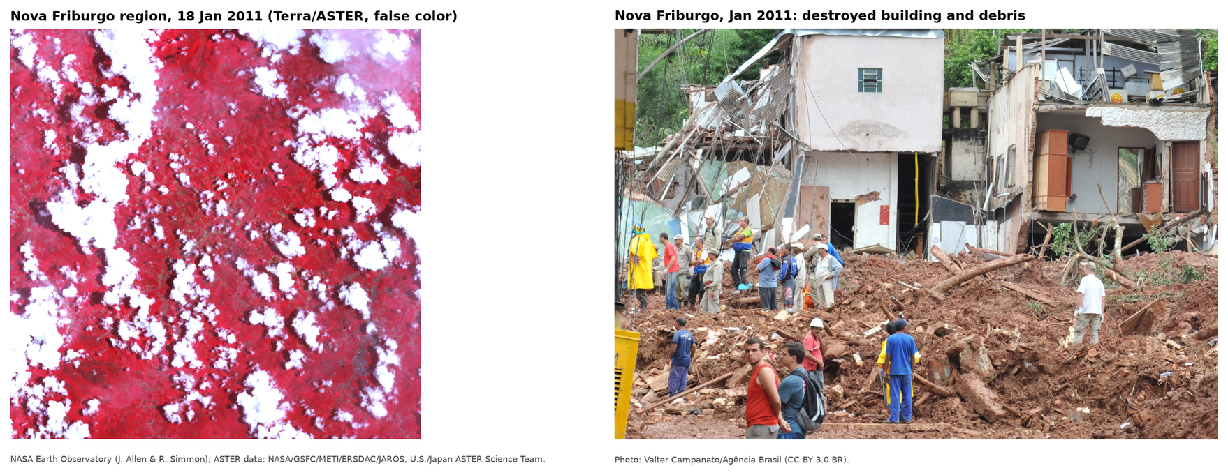
The official toll of the Rio de Janeiro State Secretariat of Civil Defense (SEDEC-RJ, integrated with the State Military Fire Brigade, CBMERJ), presented by Santos (2013), records 918 deaths in the Rio de Janeiro Highlands (Região Serrana), 429 of them in Nova Friburgo; 304,562 people were affected, and damage and losses totaled R$ 4.78 billion, 55% of them in Nova Friburgo (World Bank, 2012). A total of 3,622 scars were mapped over 421 km² of the municipality (Coelho Netto et al., 2013, cited in Marques et al., 2017). Shallow translational slides, 0.5 to 2.0 m deep, predominated, at the contact between a more permeable lateritic horizon (~10⁻⁶ m/s) and the saprolite (~10⁻⁷ m/s), and turned into debris flows in the thalwegs (Marques et al., 2017) — exactly the mechanism that TRIGRS represents (Chapter 1).
6.1.2 The São Lucas Hospital valley
São Lucas Hospital stands on Avenida Antônio Mário Azevedo (RJ-130), in the Duas Pedras neighborhood, at the foot of the north face of Morro Duas Pedras — a granite massif with a ~45° scarp and a summit at 1,360 m. In 2011, a planar failure high on the scarp (between 1,278 and 1,300 m, in a stress-relief fracture zone) evolved into a debris flow that ran down the valley, hit part of the hospital, the highway, and houses in the neighborhood, carried blocks up to 4 m across, and caused more than 20 deaths (BRASIL/MI; JICA, 2018, with the description by Pelizoni and Nunes). The 2011 regional inventory (Marc et al., 2018; Emberson et al., 2022) records this flow as a single polygon of 37,032 m² and 747 m in length, from the scarp (1,309 m) down to 902 m, 27 m from the hospital.
The valley is the case study of Appendix A of the Manual técnico para concepção de intervenções para fluxo de detritos [Technical manual for the design of debris-flow interventions] (BRASIL/MI; JICA, 2018): design rainfall with a 200-year return period (191 mm), Vdy1 = 10,873 m³, Vdy2 = 22,422 m³, woody debris Vwy = 55 m³, and a design volume of 10,928 m³. The SABO Project (MIDR/COPPE-UFRJ/JICA — the Ministry of Integration and Regional Development, the COPPE engineering institute of the Federal University of Rio de Janeiro, and JICA) detailed the solution — a closed-type (impermeable) gravity Sabo barrier, 12 m in total height, with a capacity of 11,124 m³ (JICA, 2026) — whose cornerstone, announced by the Nova Friburgo municipal government (PMNF, 2026), was laid on January 12, 2026 (Brasil 61, 2026); the start of construction was announced in June 2026 (Correio da Manhã, 2026).
6.1.3 Why this site
- Documented process: the 2011 debris flow is described in the manual, in the regional inventory, and in satellite images (Section 6.3).
- Baseline for comparison: Appendix A provides all the parameters of the GIDES method computed from field surveys — we can measure how far a study based only on open data departs from them.
- Practical relevance: this is the site of the country’s first Sabo barrier; the design volumes and discharges in this chapter can be compared directly with those of the structure.
- Calibration: five 2011 scars have their highest point inside the watershed, and the calibration window
NF_calibracao(3.84 × 3.84 km) contains 368 polygons on both faces of Morro Duas Pedras.
6.2 Defining the Sabo dam site and the reference point
6.2.1 The manual’s criterion
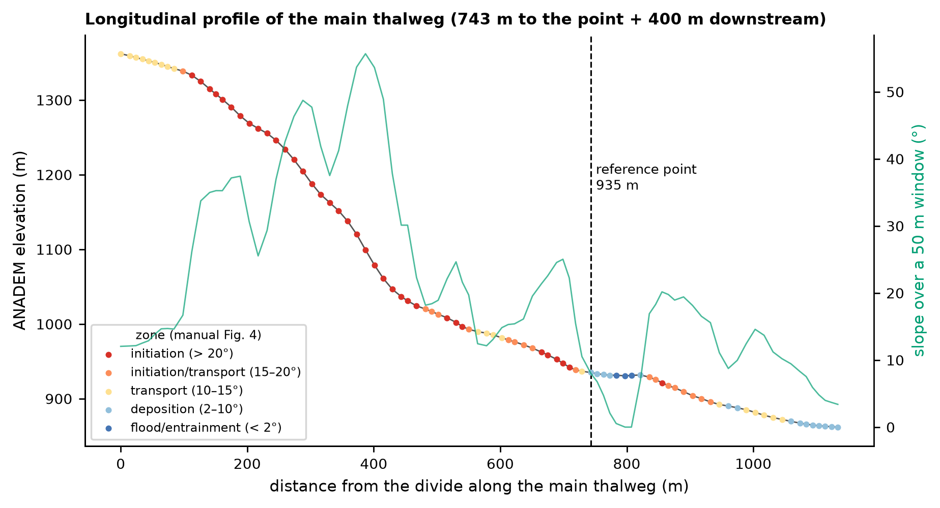
The reference point is the point on the thalweg for which volumes and discharges are computed: it lies upstream of the area to be protected and downstream of the transport (flow) zone, usually at the valley outlet, where the bed slope drops below ~10° and deposition begins (BRASIL/MI; JICA, 2018, §2.4; NILIM, 2016a, §2.4). The movement zones follow the bed slope (Fig. 4 of the manual):
| Bed slope | Zone |
|---|---|
| > 20° | initiation (generation) |
| 15° to 20° | initiation and transport |
| 10° to 15° | transport |
| 2° to 10° | deposition |
| < 2° | entrainment (hyperconcentrated flow) |
To apply the criterion to the DEM, the bed slope was computed along the D8 flow path by linear regression over a centered 50 m window (“local” slope), and also as the mean over the 200 m upstream (the slope used to compute Cd, NILIM TN 904, §2.6.3) and over the 100 m downstream. The area to be protected was identified with OpenStreetMap buildings and roads and with aggregated address counts from CNEFE 2022 (the National Address Register for Statistical Purposes of IBGE, the Brazilian Institute of Geography and Statistics), without publishing points.
6.2.2 The final point and the comparison with Appendix A
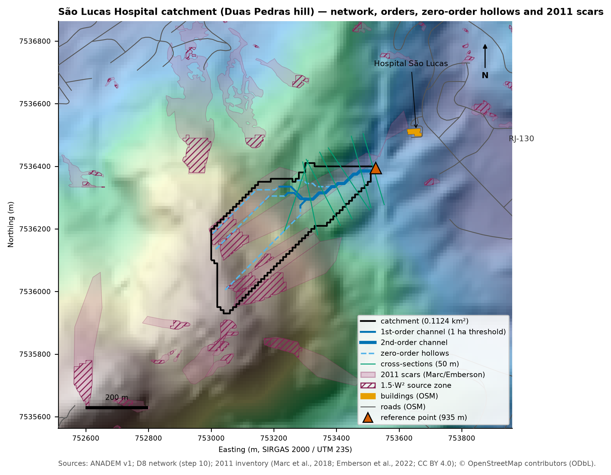
The flow path that starts at the top of the 2011 scar descends the scarp at 35–50° down to ~1,040 m, continues along the valley at 17–22° down to ~940 m and, at 935 m, enters a ~80 m bench at 2–8° (start of deposition), 189 m upstream of the hospital (Figure 6.2). The reference point was set at the start of this bench (project decision D15):
- 753,525 E; 7,536,395 N (SIRGAS 2000 / UTM 23S) = −22.259427; −42.539901 (22°15’33.94”S, 42°32’23.64”W);
- ANADEM elevation 935 m; local 50 m slope = 8.0°; mean over 200 m upstream = 16.7°; mean over 100 m downstream = 5.3°;
- 189 m upstream of the first building on the flow path (the hospital), no buildings in the watershed, and 42 CNEFE addresses in the 50 × 500 m corridor downstream;
- ~25 m from the SABO Project barrier (E 753,550; N 7,536,400; JICA, 2026);
- open cross-section, feasible for the dam: valley width of 26 m at 1 m above the bottom, 66 m at 5 m, and 90 m at 10 m, with banks of 5–9°.
data/cases/nova_friburgo/bacia/caso.json).
| Item | Appendix A (manual) | ANADEM (this study) |
|---|---|---|
| Drainage area | 0.075 km² (plan); 0.12 km² in Vdy2 | 0.1124 km² (10 m); 0.1242 km² (30 m) |
| Reference-point elevation | 910 m, valley outlet, gradient < 10° | 935 m, start of the < 10° bench |
| Main thalweg | ~800 m, predominant slope > 30% | 743 m, 57.5% (29.9°) |
| Maximum elevation | 1,360 m | 1,362 m |
| Initiation / transport / deposition | down to 1,030 m / 1,030–920 m / < 920 m | 36° scarp down to ~1,040 m / 19.6° valley (1,040–940 m) / 2–8° bench at 935–931 m |
| Width | 2.3 m in the erosion reach; Bd = 10 m at the outlet | 14–26 m in the 7 DEM cross-sections (median of 18 m; P25–P75 of 17–21 m); 26 m at the point |
The shape, area, thalweg length, and zones reproduce Appendix A; the difference lies in the elevation of the point (935 vs. 910 m). In ANADEM, 910 m corresponds to the southwest corner of the hospital, where the local slope is 19° (alternative NF-B, with 0.143 km²). The difference may come from the vertical error of the DEM in a narrow valley, from the 30 m smoothing, from terrain changes around the hospital, or from the vertical datum of the manual’s survey — it cannot be resolved without fieldwork. Both alternatives are recorded (Table 6.4).
candidatos_ponto_referencia.csv).
| Alternative | E / N (m) | Elevation (m) | Area (km²) | Slope 50 m / 200 m upstr. / 100 m downstr. (°) | 1st building downstream |
|---|---|---|---|---|---|
| Final (D15) | 753,525 / 7,536,395 | 935 | 0.112 | 8.0 / 16.7 / 5.3 | 189 m |
| NF-B (the manual’s 910 m elevation) | 753,615 / 7,536,455 | 909 | 0.143 | 19.4 / 11.3 / 13.8 | 42 m |
| NF-C (transition by the 100 m downstream mean) | 753,485 / 7,536,385 | 947 | 0.098 | 25.0 / 18.4 / 8.3 | 233 m |
WarningThe 30 m DEM does not replace a field survey
ANADEM does not resolve 2–10 m wide gullies or small structures. The bed width from the DEM (14–26 m in the cross-sections every 50 m; median of 18 m) is an upper bound: the manual measured a 2.3 m valley floor in the erosion reach and adopted Bd = 10 m at the valley outlet. In design practice, the reference point, widths, and erodible depths must be confirmed in the field (topographic survey, drone, or LiDAR).
6.3 Input datasets
Table 6.5 summarizes the layers used in the case. All of them were standardized to SIRGAS 2000 / UTM 23S (EPSG:31983), and each source has a FONTE.md (“source”) file with URL, date, license, and SHA-256 (data/raw/ and data/interim/bases/).
| Layer | Source | Resolution / scale | Reference date | License | Use in the case |
|---|---|---|---|---|---|
| DEM | ANADEM v1 (Laipelt et al., 2024) | ~30 m (resampled to 10 m) | 2011–2015 acquisitions (Copernicus GLO-30) | CC BY 4.0 | watershed, slope, profile, TRIGRS |
| Soils | IBGE BDiA (Environmental Information Database), Pedology | 1:250,000 | compilation, 2021 version | free use with attribution | hydrologic soil group (CN), zones |
| Soil texture | ISRIC SoilGrids 2.0 (Poggio et al., 2021) | 250 m | WoSIS snapshot, 2020 | CC BY 4.0 | hydraulic properties (TRIGRS) |
| Geology | SGB/UERJ, 1:100,000 maps (Nova Friburgo sheet) | 1:100,000 | — | SGB public data | property zones |
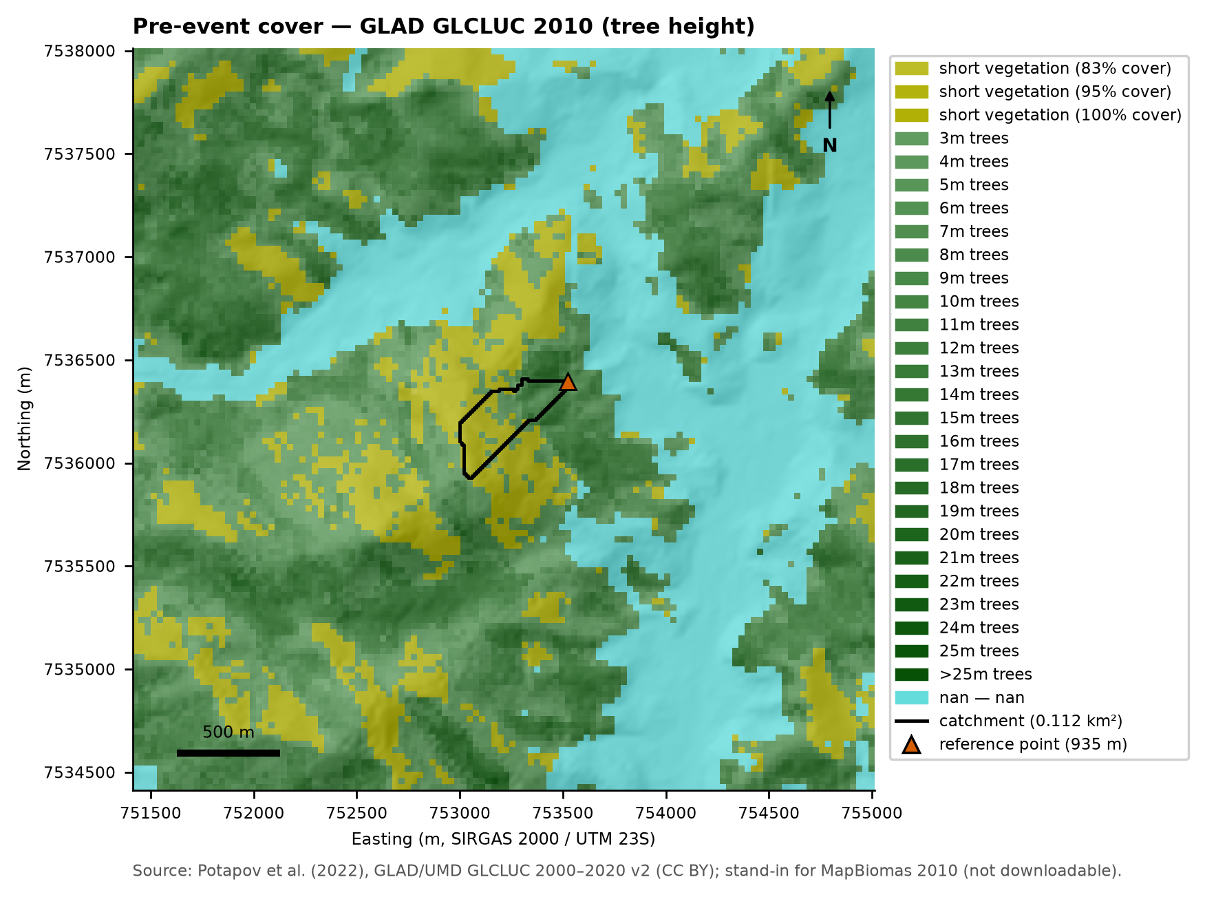
| Pre-event land cover | GLAD GLCLUC 2010 (Potapov et al., 2022) | ~30 m | 2010 | CC BY | 2010 condition; woody debris (Vwy) |
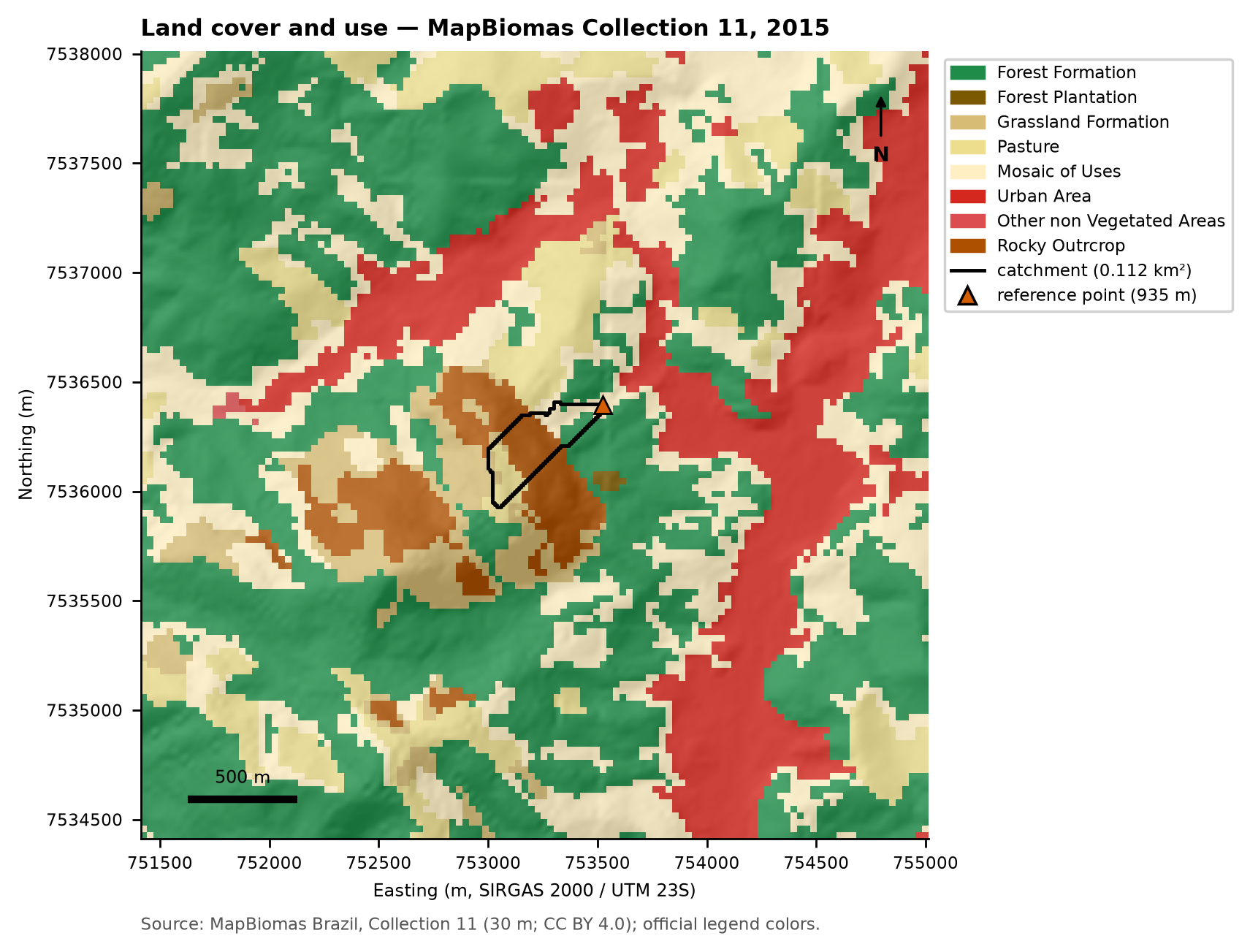
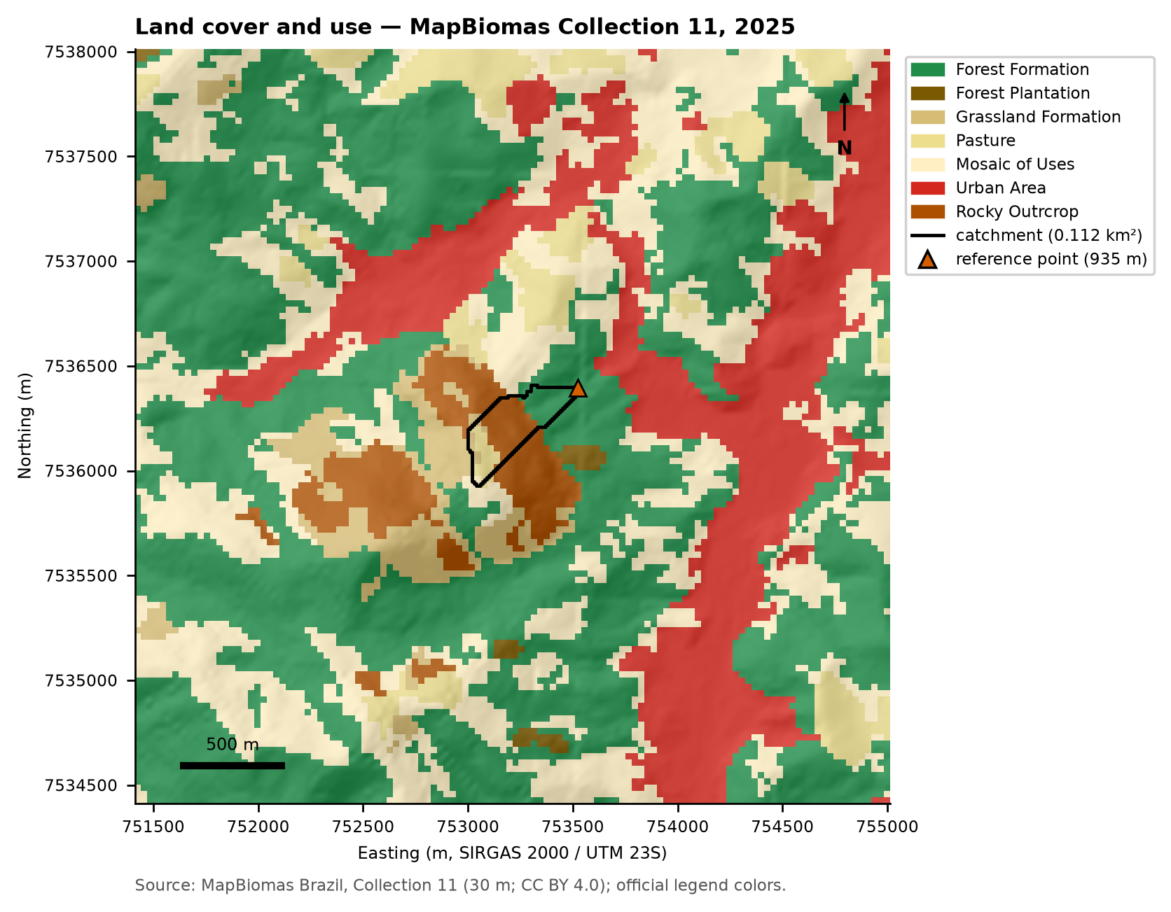
| Land cover and use | MapBiomas Collection 11 | 30 m | 2015 and 2025 | CC BY 4.0 | CN, rock outcrops (GIDES) |
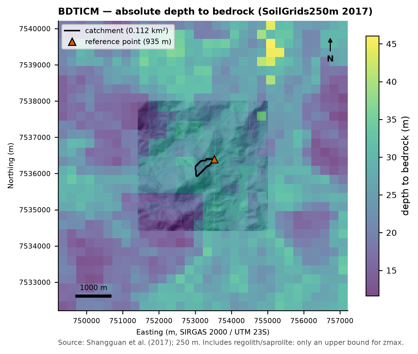
| Depth to bedrock | SoilGrids250m 2017, BDTICM (Shangguan et al., 2017) | 250 m | 2017 | ODbL | sensitivity of zmax (spatial pattern) |
| Imagery | Landsat 5 TM Collection 2 L2 (USGS) | 30 m | Sep 4, 2010 and Feb 11, 2011 | public domain | scars (calibration) |
| Scar inventory | Marc et al. (2018); Emberson et al. (2022) | polygons | 2011 event | CC BY 4.0 | method “a” of Vdy12; calibration |
| Exposure | OpenStreetMap; IBGE CNEFE 2022 | vector | Oct 30, 2026; 2022 | ODbL; free use | area to be protected |
6.3.1 DEM and relief
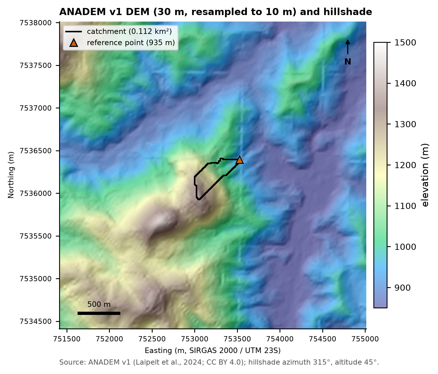
ANADEM (Laipelt et al., 2024) is a digital terrain model derived from Copernicus GLO-30 with the vegetation bias removed (mean bias of 1.5 m in the authors’ validation, versus 9.6 m for GLO-30). The 12 × 12 km window was reprojected to 30 m (bilinear) and to 10 m (bicubic) from the original. Resampling to 10 m does not create information (decision D5): it only smooths the D8 paths and the outline of a watershed that has 1,124 cells of 10 m and only 138 of 30 m. Note: the DEM postdates 2011, so the scars are already “imprinted” in the relief.
6.3.2 Slope
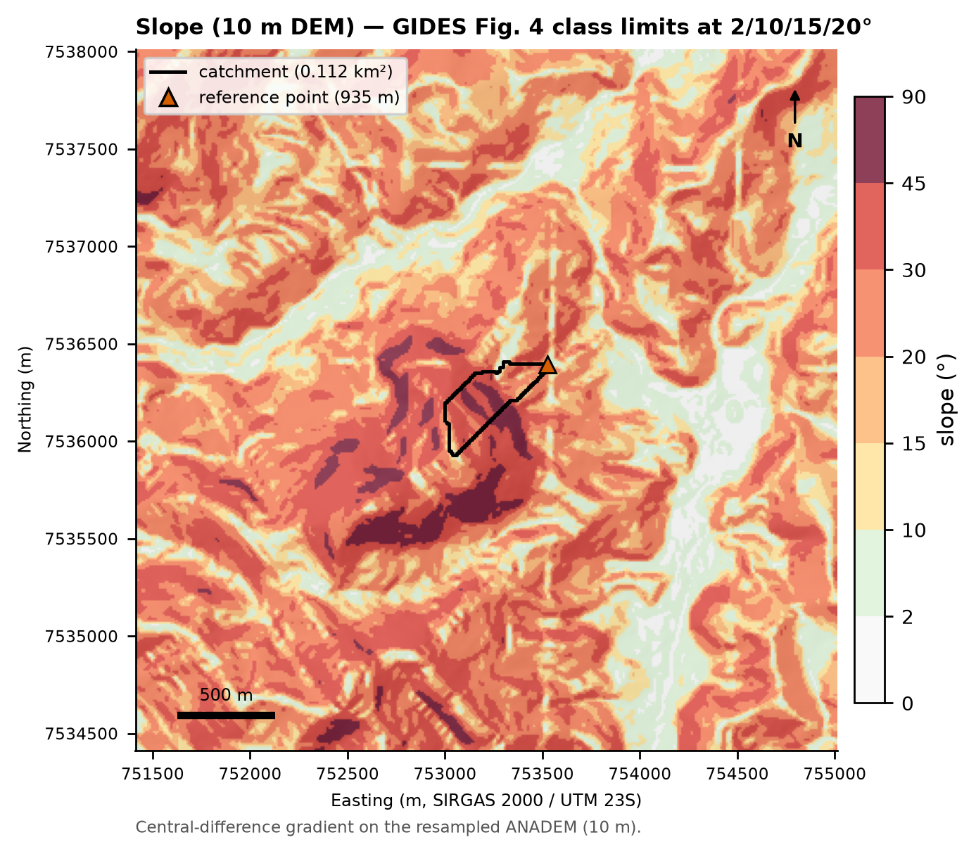
The watershed is very steep: the slope (10 m DEM) has a median of 34.4°, a P10 of 18.9°, and a P90 of 47.4°; 64% of the area exceeds 30° and 19% exceeds 45° (Figure 6.4). The classes in the figure use the limits of Fig. 4 of the manual (2°, 10°, 15°, and 20°) plus 30° and 45°.
6.3.3 D8 flow direction and contributing area
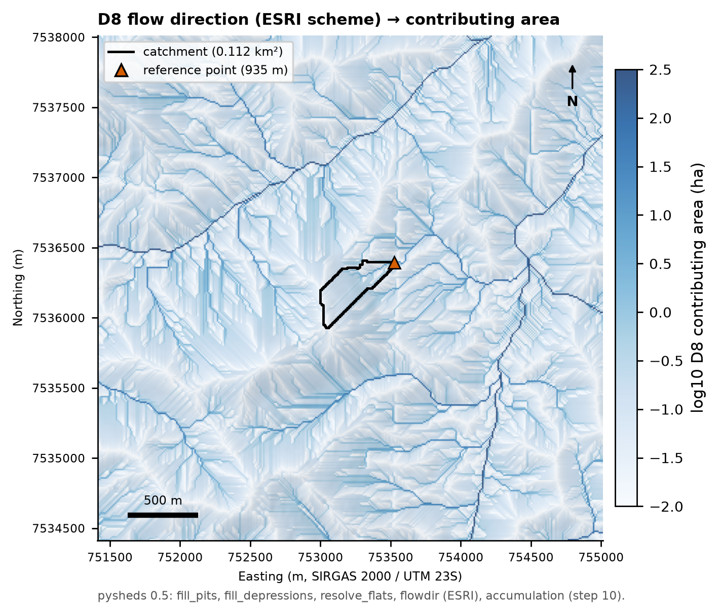
The conditioned DEM (depression filling and resolution of flat areas; Barnes et al., 2014) yields the D8 flow direction in the ESRI scheme (E = 1, SE = 2, S = 4, SW = 8, W = 16, NW = 32, N = 64, NE = 128) and the contributing area (Figure 6.5). Within the watershed, no cell was changed by more than 0.1 m by the filling. TRIGRS/TopoIndex computes its own flow direction on the model grids (Section 6.8.1).
6.3.4 Soils and texture
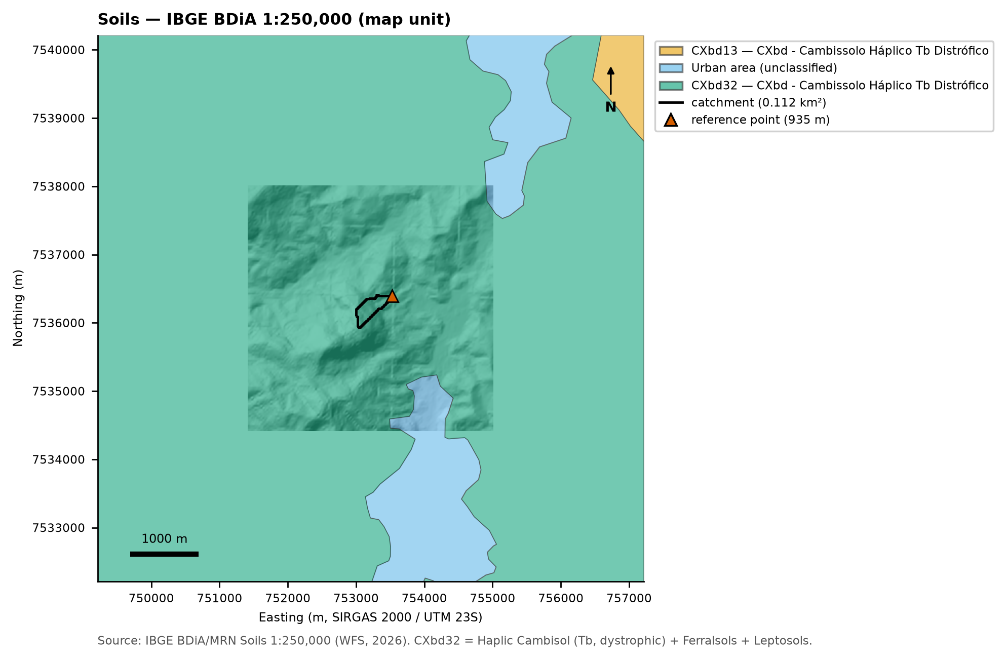
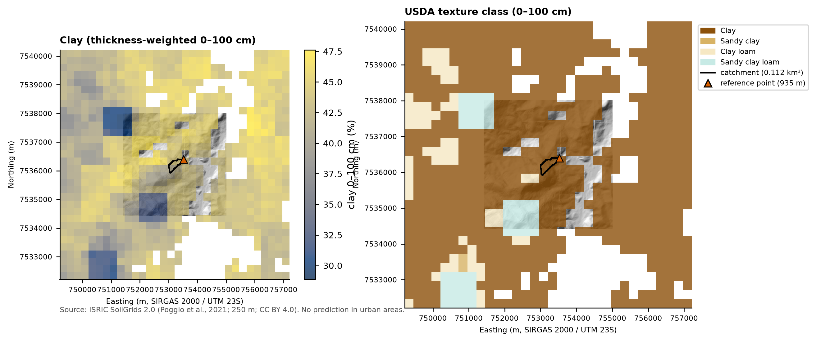
At the 1:250,000 scale, the entire watershed (100%) lies in map unit CXbd32 — Cambissolo Háplico Tb Distrófico (Brazilian Soil Classification System; roughly a dystric Cambisol), with medium and clayey texture, associated with humic Yellow and Red-Yellow Latossolos (Ferralsols) and with inclusions of Litholic Neossolos (Leptosols) (Figure 6.6). SoilGrids gives, for the six 250 m pixels that touch the watershed, an average of 42% clay and 39% sand (0–100 cm), in the Clay textural class (Figure 6.7). The nearest soil profile of RADAMBRASIL (the national radar-based natural-resources survey; profile SF23ZB/P.1, ~3 km away) is a humic Latossolo Amarelo with 440–580 g/kg of clay down to 2.3 m. For the SCS-CN method, the medium-textured Cambissolo was assigned to hydrologic soil group C (Sartori et al., 2005), with group D as a sensitivity case (Section 6.5.6).
6.3.5 Geology
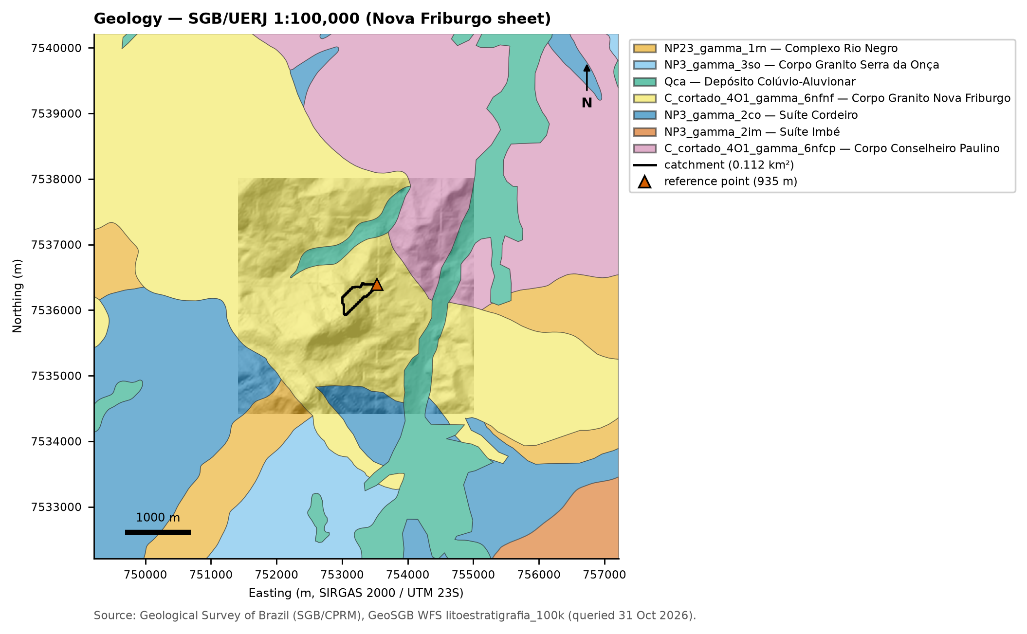
The SGB/UERJ 1:100,000 map (Nova Friburgo sheet; SGB = Geological Survey of Brazil, UERJ = State University of Rio de Janeiro) places the entire watershed in the Nova Friburgo Granite body (a post-collisional Cambro-Ordovician granite), with Quaternary colluvial–alluvial deposits (Qca) in the valley downstream (Figure 6.8). The manual describes Morro Duas Pedras as granite of the Serra dos Órgãos suite, with two families of subvertical fractures (59° and 148°) that, together with the stress-relief (sheeting) joints, form blocks and slabs (Portella et al., cited in BRASIL/MI; JICA, 2018) — the source of the boulders, up to 4 m across, carried in 2011.
6.3.6 Land use and land cover
The 2010 MapBiomas map (MapBiomas is Brazil’s annual land-cover mapping initiative) is not available without a Google Earth Engine account; as the pre-event state we used GLAD GLCLUC 2010 (Potapov et al., 2022), which separates short vegetation (by % cover) and trees (by height). In the watershed, GLAD 2010 gives 48% tree cover (trees 4 to 20 m tall) and 52% dense short vegetation (Figure 6.9). MapBiomas 2015 and 2025 (post-event) separate the rock outcrop of the scarp: 44% (2015) and 47% (2025) of the watershed, in addition to forest formation (12% → 29%), pasture (20% → 17%), grassland (5.5%), and mosaic of uses (19% → 1%) (Figure 6.10, Figure 6.11). The outcrop is decisive at two points in this chapter: it raises the watershed’s CN and it has no erodible material for Vdy1.
6.3.7 Depth to bedrock
BDTICM (Shangguan et al., 2017) indicates a depth to bedrock of 25.7 to 29.1 m in the watershed (Figure 6.12). This value refers to regolith/saprolite, not to mobilizable soil: the 2011 landslides were 0.5–2.0 m deep (Marques et al., 2017), and the manual describes shallow soil over rock on the scarp. BDTICM therefore does not set the depth of the TRIGRS impermeable base (zmax, at most 5 m): it enters only the sensitivity analysis, as an alternative spatial pattern of soil thickness (Section 6.8.3).
NoteProperty zones,
zmax, and initial water table
The TRIGRS-specific grids — property zones (geology × land cover), zmax (an exponential function of slope, calibratable, between 0.3 and 5 m, with lower caps on the rock outcrop and on the shallow soil), and the initial water-table scenarios depthwt = min(d, zmax) with d = 1, 2, …, 10 m (decision D6) — are presented together with the model parameterization, in Section 6.8.
6.3.8 Satellite images before and after the event
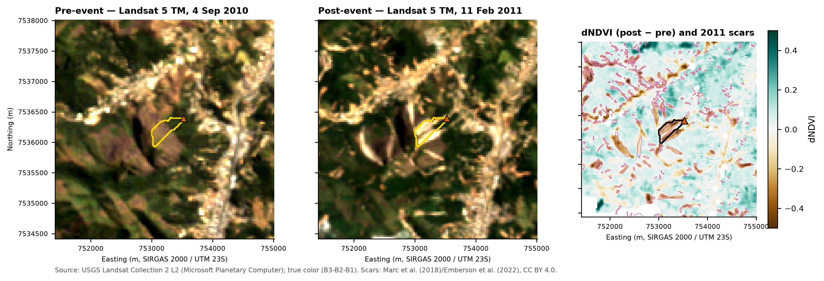
The Landsat 5 TM pair of September 4, 2010 (pre-event) and February 11, 2011 (post-event) is the cleanest available (99.9% and 76.3% usable pixels within the ±6 km window). The scars show up as fresh bare soil and a drop in NDVI (Figure 6.13). Against the 2011 inventory, the bare-soil rule (dNDVI < −0.20, post-event NDVI < 0.35, slope ≥ 15°) has a precision of 0.867 and a recall of 0.207 (F1 = 0.334): it is right where it flags, but it only captures the large scars (52% of the scars ≥ 3,600 m² and 1.4% of those < 900 m²). In Nova Friburgo, unlike Teresópolis, the inventory does not need to be shifted (decision D17).
6.4 Watershed delineation and drainage network
6.4.1 Step by step
- DEM conditioning (pysheds 0.5):
fill_pits→fill_depressions→resolve_flats. - D8 flow direction (ESRI scheme) and flow accumulation (number of cells that drain to each cell).
- Watershed: all cells that drain to the reference point (10 m); polygon obtained by vectorizing the mask.
- Main thalweg: the longest D8 flow path, from the divide to the point (used for L, S, and Tc).
- Start of the first-order channels: the manual defines order zero from the contour lines (“a” greater than “b”) and the start of the first order where a = b (Fig. 12 of the manual; NILIM, 2016a, §2.6.1). Tested along the thalweg with the contours of the 10 m DEM, the criterion is never met (maximum b/a of 0.29): at 30 m resolution the gullies do not show up. We therefore adopted a contributing-area threshold of 1 ha, calibrated on Appendix A itself: it yields 479 m of channels (the manual cites a first-order thalweg of ~500 m) and places the channel head at 1,037 m, at the foot of the scarp, where the manual ends the initiation zone (1,030 m).
- Strahler order (Strahler, 1957) on the watershed network and zero-order thalwegs: from the channel heads up to the divide (“headwater”) and lateral valleys that reach a channel (A ≥ 0.25 ha and convergence A/L ≥ 30 m).
6.4.2 Watershed metrics
The time of concentration was computed for the main thalweg (L = 0.7433 km; S = 0.5746 m/m) with three formulas (Silveira, 2005):
\[ t_c^{\text{Kirpich}} = 0.0195\,L^{0.77}S^{-0.385}\ \text{[min; L in m]},\qquad t_c^{\text{Giandotti}} = \frac{4\sqrt{A}+1.5L}{0.8\sqrt{H_m}}\ \text{[h]},\qquad t_c^{\text{Ven Te Chow}} = 0.1602\left(\frac{L}{\sqrt{S}}\right)^{0.64}\ \text{[h; L in km]} \]
with \(H_m\) = mean elevation − outlet elevation (211.1 m).
caso.json, step 10).
| Metric | Value | Metric | Value |
|---|---|---|---|
| Area (10 m / 30 m) | 0.1124 / 0.1242 km² | Main thalweg | 743.3 m (1,362 → 934.9 m) |
| Perimeter | 2.04 km | Thalweg slope | 0.5746 m/m (57.5%; 29.9°) |
| Compactness coefficient Kc | 1.70 | Tc Kirpich | 3.92 min |
| Form factor Kf | 0.203 | Tc Ven Te Chow | 9.49 min |
| Min. / mean / max. elevation | 934.9 / 1,146.1 / 1,362.1 m | Tc Giandotti | 12.68 min |
| Relief | 427.2 m | Channel threshold | 1 ha |
| Mean watershed slope | 34.1° (71.8%) | Channel heads / maximum order | 3 / 2 |
| Area with slope > 30° | 64% | Ldy11 (order ≥ 1) | 478.7 m (order 1: 207.3; order 2: 271.4) |
| 2011 scars touching the watershed | 5 (58,399 m² inside the watershed) | Ldy12 (order zero) | 1,040.2 m (headwater 922.0 + lateral 118.3) |
| Buildings in the watershed | 0 | Drainage density | 4.26 km/km² |
The spread among the Tc formulas (a factor of ~3) is typical of small, steep watersheds (Silveira, 2005); the choice is made in Section 6.5.6. The 2011 polygons cover 52% of the area because they include the track and the deposit of the flow, not only the failures.
6.4.3 Sensitivity to the channel threshold
| Threshold (ha) | Channel heads | Max. order | Ldy11 (m) | Ldy12 (m) | Ldy11 + Ldy12 (m) |
|---|---|---|---|---|---|
| 0.25 | 18 | 3 | 2,421.9 | 5,268.7 | 7,690.6 |
| 0.5 | 8 | 2 | 687.7 | 3,268.1 | 3,955.8 |
| 1 | 3 | 2 | 478.7 | 1,040.2 | 1,518.9 |
| 2 | 1 | 1 | 281.4 | 1,237.5 | 1,518.9 |
| 3 | 1 | 1 | 271.4 | 878.8 | 1,150.2 |
| 5 | 1 | 1 | 261.4 | 491.1 | 752.5 |
With the 2 ha threshold a single first-order channel remains, as in the manual, but 281 m long. Since Vdy11 and Vdy12 use the same Bd·De in method “b” (Section 6.7), the sum Vdy1 is hardly sensitive to the threshold between 1 and 2 ha; the split between bed (order ≥ 1) and hillslope (order zero), however, is.
locacao.py (excerpt) — watershed and network with pysheds
import numpy as np
from pysheds.grid import Grid
np.in1d = np.isin  # pysheds 0.5 still calls np.in1d (removed in NumPy 2)

grid = Grid.from_raster("mde_janela_10m_bicubico.tif")
dem = grid.read_raster("mde_janela_10m_bicubico.tif")
dem = grid.resolve_flats(grid.fill_depressions(grid.fill_pits(dem)))
dirmap = (64, 128, 1, 2, 4, 8, 16, 32)            # ESRI scheme: N, NE, E, SE, S, SW, W, NW
fdir = grid.flowdir(dem, dirmap=dirmap)
acc = grid.accumulation(fdir, dirmap=dirmap)       # no. of cells (includes the cell itself)

x, y = 753525.0, 7536395.0                          # reference point (EPSG:31983)
bacia = grid.catchment(x=x, y=y, fdir=fdir, dirmap=dirmap, xytype="coordinate")
canais = acc * 100.0 >= 10_000.0                    # 1 ha threshold with 10 m cells
6.5 Design rainfall
Rainfall enters the chain twice: as the design maximum daily rainfall Pd(T) in Equation 6 of the manual (Vdy2) and as a hyetograph in TRIGRS and in the hydrograph. This section builds both from the daily series of HIDRO/ANA in the DPM database (data up to February 28, 2026; identical to ANA’s web service on the common dates).
6.5.1 Rain gauges
Within a 40 km radius there are 41 rain gauges with data; 23 have 30 or more valid years. Table 6.8 lists the stations used: the reference trio recommended by the data step (the manual’s gauge, the closest one, and the longest record) and the other stations with ≥ 30 valid years within 20 km of the point (the “envelope”), used in the regional analysis (Figure 6.15). Distances are to the final reference point; the inventory elevation differs from the ANADEM elevation because the old coordinates were rounded to the minute.
| Code | Station | Owner/operator | Dist. (km) | Elev. inventory/ANADEM (m) | Record (valid years) | n | Missing (%) | Last record | x̄ max. (mm) | g | Role |
|---|---|---|---|---|---|---|---|---|---|---|---|
| 02242020 | Vargem Grande | ANA/SGB-CPRM | 4.1 | 680 / 989 | 1966–2025 | 60 | 0.22 | 2026-02-28 | 81.1 | 1.53 | ref. 2 (closest) |
| 02242023 | Conselheiro Paulino | ANA/ANA | 5.3 | 830 / 873 | 1939–1982 | 43 | 0.23 | 1983-04-22 | 79.7 | 0.72 | envelope |
| 02242025 | Cascatinha do Cônego | ANA/SGB-CPRM | 9.4 | 1,210 / 1,198 | 1968–2025 | 55 | 2.19 | 2026-02-28 | 82.6 | 0.54 | ref. 1 (manual) |
| 02242022 | Fazenda Mendes | ANA/SGB-CPRM | 12.7 | 1,010 / 1,019 | 1950–2025 | 76 | 0.19 | 2026-02-28 | 75.0 | 1.92 | ref. 3 (longest record) |
| 02242024 | Teodoro de Oliveira | ANA/SGB-CPRM | 13.1 | 1,105 / 1,065 | 1966–2025 | 60 | 0.00 | 2026-02-28 | 124.6 | 2.47 | envelope (escarpment) |
| 02242019 | Vargem Alta | ANA/SGB-CPRM | 15.0 | 1,100 / 1,016 | 1966–2025 | 60 | 0.02 | 2026-02-28 | 85.8 | 2.18 | envelope |
| 02242005 | Fazenda São João | ANA/SGB-CPRM | 15.2 | 960 / 974 | 1968–2025 | 58 | 0.14 | 2026-02-28 | 113.1 | 1.50 | envelope (escarpment) |
| 02242021 | Bom Jardim | ANA/SGB-CPRM | 17.1 | 530 / 554 | 1941–2025 | 81 | 1.74 | 2026-02-28 | 76.3 | 0.91 | envelope |
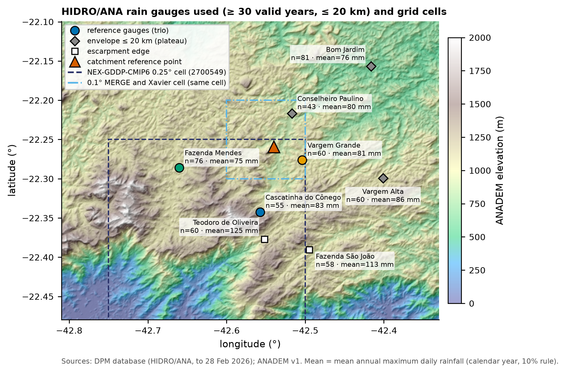
Orographic variability is strong. The stations on the edge of the Serra do Mar escarpment, south of the city (Teodoro de Oliveira and Fazenda São João), have annual totals of 3,306 and 2,133 mm and mean annual maxima of 125 and 113 mm; those on the plateau, where the watershed lies, have 1,325–1,531 mm per year (Cascatinha do Cônego, at 1,198 m, reaches 2,170 mm) and mean annual maxima of 75 to 86 mm. The São Lucas Hospital watershed is on the plateau (the escarpment-edge stations are 13–15 km away), between Vargem Grande (4 km) and Conselheiro Paulino (5 km; record ended in 1983).
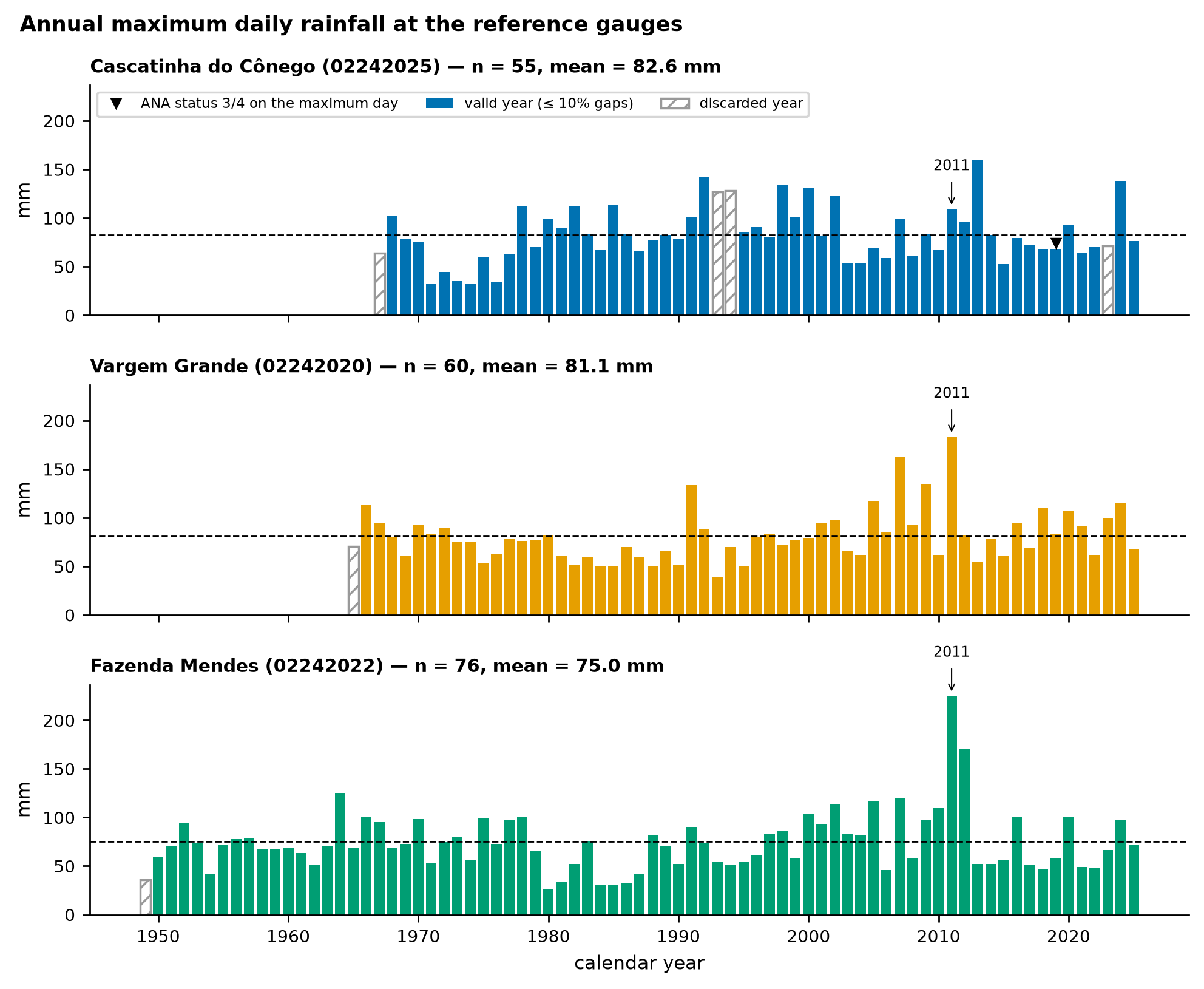
6.5.2 Annual maximum series and quality control
Rules (the same for all stations):
- valid daily value: ≥ 0; missing = nulls, negatives, and −99999;
- the reading of day D is taken at 07:00 and covers the previous 24 h (HIDRO convention);
- calendar year (as in the manual) and October–September hydrological year, for comparison;
- a year is accepted with up to 10% missing days (a rule that, in practice, reproduces the manual’s selection); 2026 excluded;
- maxima whose day has ANA status 3 (doubtful) or 4 (accumulated) are flagged and tested as a sensitivity case.
| Station | Year type | Years with data | Valid years (≤ 10%) | Complete | Maxima with status 3/4 | Mean (mm) | Std. dev. (mm) | Largest maximum (year) |
|---|---|---|---|---|---|---|---|---|
| Cascatinha do Cônego | calendar | 59 | 55 | 48 | 1 | 82.6 | 28.1 | 160.3 (2013) |
| Cascatinha do Cônego | hydrological (Oct–Sep) | 60 | 55 | 49 | 1 | 79.8 | 28.0 | 160.3 (2012) |
| Vargem Grande | calendar | 61 | 60 | 57 | 0 | 81.1 | 27.0 | 183.5 (2011) |
| Vargem Grande | hydrological (Oct–Sep) | 61 | 59 | 56 | 0 | 80.2 | 27.7 | 183.5 (2010) |
| Fazenda Mendes | calendar | 77 | 76 | 73 | 0 | 75.0 | 30.8 | 225.4 (2011) |
| Fazenda Mendes | hydrological (Oct–Sep) | 78 | 76 | 73 | 0 | 75.5 | 30.6 | 225.4 (2010) |
Two diagnostics from the data step (06_chuva.md) guide the use of the series:
- Trend: none of the reference stations has a significant trend at 5% over the full period (Mann–Kendall with tie correction); within the 40 km radius the signals are mixed, and only 2 of 40 stations survive the false-discovery-rate control. The stationarity hypothesis is kept for the present climate; climate change enters through the CMIP6 factors (Section 6.6).
- Homogeneity of Cascatinha do Cônego: the ratio between Cascatinha and four neighbors drops from 2001–2002 onward (Pettitt test: p = 0.0002 for the annual totals; p = 0.056 for the maxima). For this reason this station — the manual’s — is not used on its own.
6.5.3 Statistical fitting and choice of the design rainfall
6.5.3.1 Step 1 — reproduce the manual
Appendix A fitted the Gumbel distribution by the method of moments to the 46 values of Table 4.1 (Cascatinha do Cônego, 1967–2015), because the skewness g = 0.378 < 1.5 (criterion of the Manual de Inventário Hidroelétrico [Hydropower Inventory Manual], which recommends the 2-parameter exponential if g > 1.5):
\[ \alpha = 0.779\,s, \qquad \beta = \bar{x} - 0.577\,\alpha, \qquad x_T = \beta - \alpha\,\ln\!\left[-\ln\!\left(1 - \tfrac{1}{T}\right)\right]. \]
With the same values — x̄ = 83.48 mm, s = 29.317 mm, α = 22.84 mm, and β = 70.31 mm — we obtain P100 = 175.4 mm and P200 = 191.2 mm (manual: 175 and 191 mm; the 16 published quantiles are reproduced to the millimeter). The data step showed that 44 of the 46 values are raw (not quality-controlled) ANA maxima. With the updated series from the database (1968–2025, 55 years, 10% rule), the same method gives 170.7 mm (T = 100 years) and 185.9 mm (T = 200 years).
6.5.3.2 Step 2 — at-site fitting at the three reference stations
For each station we fitted seven distributions by up to four methods with trigrs_mapper.hydro.frequencia (Gumbel, 2-parameter exponential, GEV, Pearson III, log-Pearson III, and 2- and 3-parameter log-normal; moments, L-moments, and maximum likelihood, ML), with goodness-of-fit tests (Kolmogorov–Smirnov, Anderson–Darling, chi-square, and PPCC) and the Akaike information criterion (AIC). Because the parameters are estimated from the sample itself, the classical p-values are optimistic: those in the table () come from 200 samples simulated from the fitted distribution, refitted each time (parametric bootstrap*; Efron, 1979).
| Station | Distribution (method) | AIC | p KS* | p AD* | r PPCC | p PPCC* | P100 (mm) | P200 (mm) | P500 (mm) |
|---|---|---|---|---|---|---|---|---|---|
| Cascatinha do Cônego | Gumbel (moments (manual)) | 527.0 | 0.80 | 0.26 | 0.991 | 0.58 | 170.7 | 185.9 | 206.0 |
| Cascatinha do Cônego | Gumbel (L-moments) | 526.1 | 0.60 | 0.19 | 0.991 | 0.58 | 173.7 | 189.5 | 210.3 |
| Cascatinha do Cônego | Gumbel (ML) | 525.3 | 0.48 | 0.22 | 0.991 | 0.58 | 181.8 | 198.9 | 221.3 |
| Cascatinha do Cônego | Exponential 2p (moments) | — | 0.21 | 0.06 | 0.959 | 0.06 | 183.9 | 203.4 | 229.2 |
| Cascatinha do Cônego | GEV (L-moments) | 525.5 | 0.44 | 0.25 | 0.994 | 0.55 | 161.4 | 171.8 | 184.5 |
| Cascatinha do Cônego | GEV (ML) | 525.3 | 0.41 | 0.35 | 0.993 | 0.44 | 156.6 | 165.4 | 175.8 |
| Cascatinha do Cônego | LN2 (ML) | 526.0 | 0.39 | 0.13 | 0.991 | 0.54 | 178.8 | 195.5 | 217.8 |
| Cascatinha do Cônego | LN3 (L-moments) | 525.5 | 0.47 | 0.26 | 0.994 | 0.58 | 162.3 | 174.0 | 189.0 |
| Cascatinha do Cônego | Pearson III (L-moments) | 525.6 | 0.44 | 0.27 | 0.993 | 0.52 | 161.3 | 172.3 | 186.2 |
| Cascatinha do Cônego | Log-Pearson III (L-moments) | 525.5 | 0.27 | 0.19 | 0.992 | 0.41 | 156.4 | 165.2 | 175.7 |
| Vargem Grande | Gumbel (moments (manual)) | 551.6 | 0.68 | 0.58 | 0.986 | 0.30 | 165.8 | 180.4 | 199.7 |
| Vargem Grande | Gumbel (L-moments) | 551.0 | 0.73 | 0.60 | 0.986 | 0.30 | 163.4 | 177.6 | 196.4 |
| Vargem Grande | Gumbel (ML) | 550.6 | 0.78 | 0.70 | 0.986 | 0.30 | 157.9 | 171.3 | 188.9 |
| Vargem Grande | Exponential 2p (moments) | — | 0.21 | 0.07 | 0.989 | 0.52 | 178.5 | 197.2 | 221.9 |
| Vargem Grande | GEV (L-moments) | 551.8 | 0.35 | 0.56 | 0.994 | 0.72 | 175.3 | 195.7 | 224.8 |
| Vargem Grande | GEV (ML) | 551.7 | 0.48 | 0.63 | 0.993 | 0.72 | 173.0 | 192.5 | 220.1 |
| Vargem Grande | LN2 (ML) | 551.8 | 0.68 | 0.48 | 0.981 | 0.17 | 155.6 | 167.7 | 183.6 |
| Vargem Grande | LN3 (L-moments) | 552.0 | 0.32 | 0.50 | 0.993 | 0.61 | 172.8 | 191.2 | 216.6 |
| Vargem Grande | Pearson III (L-moments) | — | 0.29 | 0.23 | 0.989 | 0.33 | 168.2 | 183.0 | 202.2 |
| Vargem Grande | Log-Pearson III (L-moments) | 551.8 | 0.40 | 0.55 | 0.993 | 0.63 | 172.5 | 191.4 | 217.9 |
| Fazenda Mendes | Gumbel (moments (manual)) | 718.2 | 0.47 | 0.35 | 0.969 | 0.06 | 171.6 | 188.3 | 210.4 |
| Fazenda Mendes | Gumbel (L-moments) | 717.5 | 0.72 | 0.43 | 0.969 | 0.06 | 166.5 | 182.3 | 203.2 |
| Fazenda Mendes | Gumbel (ML) | 717.5 | 0.75 | 0.45 | 0.969 | 0.06 | 165.5 | 181.2 | 201.8 |
| Fazenda Mendes | Exponential 2p (moments) | — | 0.17 | 0.13 | 0.966 | 0.07 | 186.2 | 207.5 | 235.8 |
| Fazenda Mendes | GEV (L-moments) | 719.3 | 0.54 | 0.24 | 0.972 | 0.03 | 170.2 | 187.8 | 211.5 |
| Fazenda Mendes | GEV (ML) | 719.3 | 0.58 | 0.27 | 0.972 | 0.03 | 171.6 | 189.6 | 214.0 |
| Fazenda Mendes | LN2 (ML) | 717.6 | 0.68 | 0.34 | 0.970 | 0.06 | 168.6 | 185.4 | 207.9 |
| Fazenda Mendes | LN3 (L-moments) | 719.7 | 0.50 | 0.18 | 0.970 | 0.03 | 168.7 | 185.6 | 208.4 |
| Fazenda Mendes | Pearson III (L-moments) | 723.4 | 0.40 | 0.13 | 0.966 | 0.00 | 165.4 | 179.9 | 198.5 |
| Fazenda Mendes | Log-Pearson III (L-moments) | 720.1 | 0.53 | 0.20 | 0.965 | 0.01 | 160.8 | 174.8 | 193.0 |
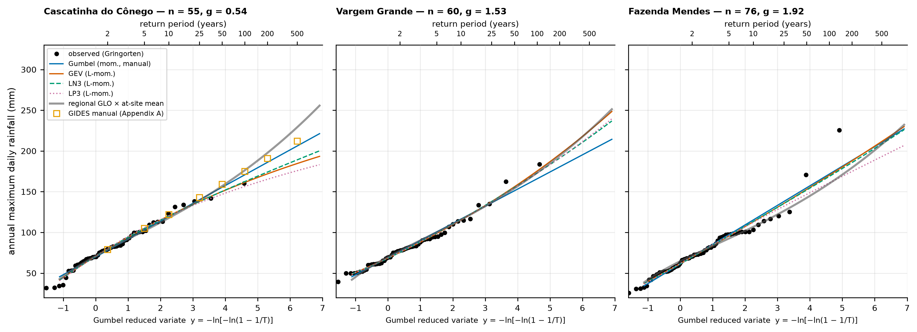
Reading Table 6.10 and Figure 6.17:
- No distribution is rejected by the Kolmogorov–Smirnov and Anderson–Darling tests at 5% (PPCC rejects GEV, LN3, Pearson III, and log-Pearson III at Fazenda Mendes, which are sensitive to the 2011 value of 225.4 mm), and the AIC differences among the best candidates are smaller than 2 — with 55 to 76 years of data, the sample cannot distinguish among the families.
- Even so, the high-T quantiles diverge: at Cascatinha, from 156 mm (log-Pearson III) to 182 mm (Gumbel by ML) for T = 100 years, or 184 mm with the 2-parameter exponential, which the manual’s criterion does not recommend there (g = 0.54 < 1.5). Under the manual’s criterion, Vargem Grande (g = 1.53) and Fazenda Mendes (g = 1.92) would already be fitted with the 2-parameter exponential, with 178–186 mm for T = 100 years.
- The at-site 90% confidence intervals (nonparametric bootstrap, 1,000 replicates; Efron, 1979) for T = 100 years under GEV are ~50–90 mm wide (Cascatinha 135.5–183.2 mm; Vargem Grande 133.9–215.7 mm; Fazenda Mendes 129.1–222.2 mm).
Conclusion: at-site fitting is unstable for T ≥ 100 years. The classical way out is to regionalize: use the several stations of a homogeneous region to estimate the shape of the distribution.
6.5.3.3 Step 3 — regional analysis by L-moments
L-moments are linear combinations of the ordered observations (Hosking, 1990): λ1 (mean), λ2 (scale), and the ratios L-CV \(t = \lambda_2/\lambda_1\), L-skewness \(\tau_3 = \lambda_3/\lambda_2\), and L-kurtosis \(\tau_4 = \lambda_4/\lambda_2\). They are much less sensitive to extreme values than conventional moments. The index-flood method (Hosking and Wallis, 1997) assumes that, in a homogeneous region, the distribution at each station is the same dimensionless curve \(q(T)\) multiplied by a local index (the mean of the annual maxima):
\[ P_d(T) = \mu \cdot q(T). \]
Three statistics decide the region and the distribution (Hosking and Wallis, 1997):
- Discordancy \(D_i\) of each station relative to the group, in the (t, τ3, τ4) space — critical value 2.140 for 8 stations and 1.648 for 6;
- Heterogeneity \(H_1 = (V - \mu_V)/\sigma_V\), where V is the weighted dispersion of L-CV among stations and \(\mu_V\), \(\sigma_V\) come from 500 regions simulated from a 4-parameter kappa distribution (Hosking, 1994) with the same mean ratios and the same record lengths; H < 1 = acceptably homogeneous;
- Goodness of fit \(Z^{DIST} = (\tau_4^{DIST} - t_4^R + B_4)/\sigma_4\) for GLO (generalized logistic), GEV, GNO (generalized normal = LN3), PE3, and GPA (generalized Pareto); \(|Z| \le 1.64\) = accepted.
| Station | n | λ1 (mm) | L-CV t | τ3 | τ4 | D_i (R1) | D_i (R2) |
|---|---|---|---|---|---|---|---|
| Conselheiro Paulino | 43 | 79.7 | 0.195 | 0.123 | 0.150 | 0.51 | 0.43 |
| Teodoro de Oliveira | 60 | 124.6 | 0.165 | 0.254 | 0.299 | 1.31 | — (not in R2) |
| Vargem Alta | 60 | 85.8 | 0.191 | 0.107 | 0.364 | 2.12 | 1.64 |
| Fazenda São João | 58 | 113.1 | 0.169 | 0.181 | 0.197 | 0.28 | — (not in R2) |
| Bom Jardim | 81 | 76.3 | 0.165 | 0.104 | 0.141 | 1.31 | 1.08 |
| Cascatinha do Cônego | 55 | 82.6 | 0.190 | 0.107 | 0.177 | 0.38 | 0.29 |
| Vargem Grande | 60 | 81.1 | 0.175 | 0.230 | 0.201 | 0.58 | 1.50 |
| Fazenda Mendes | 76 | 75.0 | 0.210 | 0.187 | 0.196 | 1.51 | 1.06 |
| regional mean R1 | 493 | — | 0.182 | 0.162 | 0.215 | — | — |
| regional mean R2 | 375 | — | 0.187 | 0.144 | 0.204 | — | — |
| Region | Gauges | Critical D | H1 | Mean ρ | Z GLO | Z GEV | Z GNO | Z PE3 | Z GPA |
|---|---|---|---|---|---|---|---|---|---|
| R1 | 8 | 2.140 | -0.47 | 0.22 | -2.35 | -4.22 | -4.39 | -4.94 | -8.27 |
| R2 | 6 | 1.648 | -0.33 | 0.30 | -1.61 | -3.36 | -3.41 | -3.81 | -7.05 |
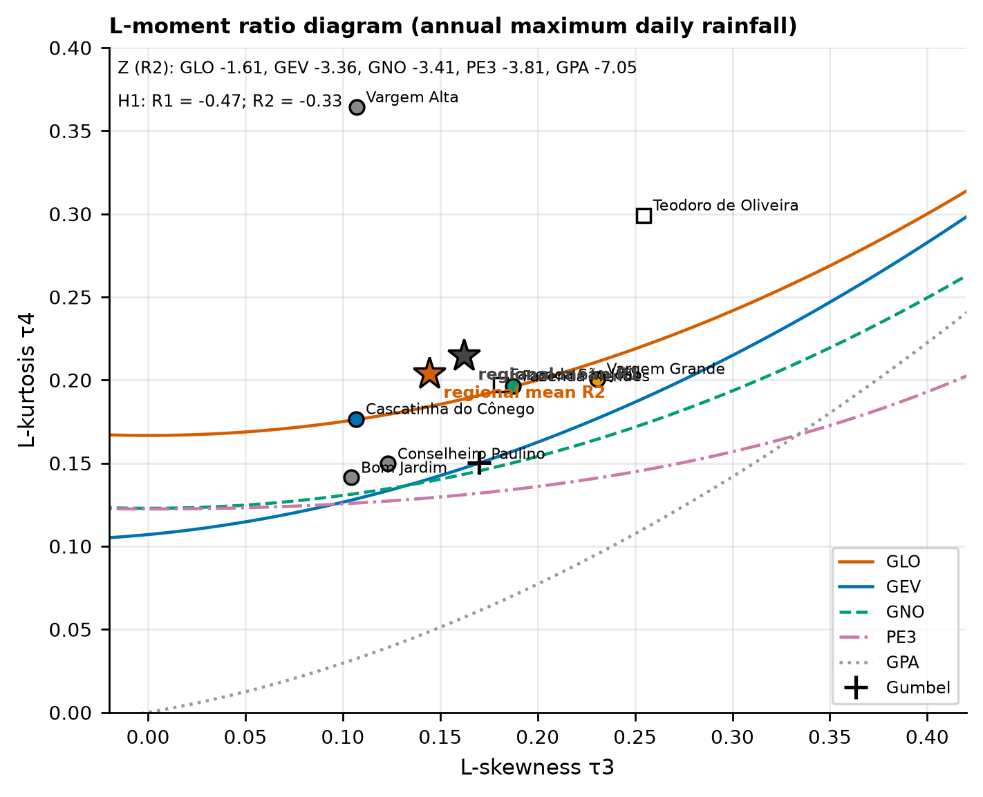
The eight stations form a region that is homogeneous in L-CV (H1 = −0.47), with no discordant station, but no distribution passes the Z test (the best one, GLO, has Z = −2.35): the two escarpment-edge stations have high L-skewness and L-kurtosis and a different rainfall regime. Without them (region R2, 6 stations and 375 station-years), the region remains homogeneous (H1 = −0.33) and GLO is the only accepted distribution (Z = −1.61). Vargem Alta is at the discordancy limit (D = 1.64 against the critical value of 1.648) because of the 271.5 mm of 2011 — it was kept, since these are real data from the event of interest.
NoteNegative H and inter-site correlation
H1 < 0 indicates an L-CV dispersion smaller than that of independent stations — expected when the maxima of neighboring stations are correlated (here, mean ρ = 0.30 in R2). With inter-site correlation, |Z| tends to be overestimated (Hosking and Wallis, 1997), so GEV and GNO, narrowly rejected, are kept as sensitivity cases in Table 6.13.
6.5.3.4 Step 4 — choice and Pd(T) table
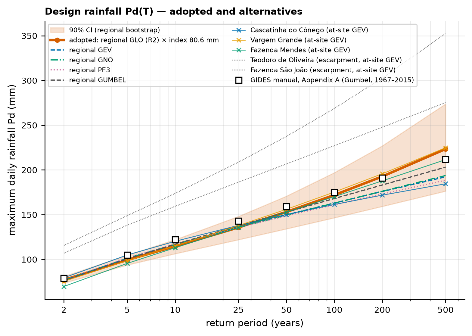
Distribution: regional GLO (R2), estimated from the regional L-moments (t = 0.187; τ3 = 0.144):
\[ q(F) = \xi + \frac{\alpha}{k}\left[1 - \left(\frac{1-F}{F}\right)^{k}\right], \qquad F = 1 - \frac{1}{T}, \]
with k = −τ3 = −0.1443, α = 0.1807, and ξ = 0.9561 (dimensionless curve, mean 1). For T = 100 years: \(q = 0.9561 + \frac{0.1807}{-0.1443}\,[1 - (0.01/0.99)^{-0.1443}] = 2.134\).
Local index: the mean of the annual maxima at the point, interpolated by inverse squared distance from the means of the six R2 stations: μ = 80.6 mm (weights: Vargem Grande 0.49; Conselheiro Paulino 0.30; Cascatinha do Cônego 0.10; Fazenda Mendes 0.05; Vargem Alta 0.04; Bom Jardim 0.03).
Uncertainty: 90% interval by regional bootstrap — 2,000 replicates in which the years are resampled with replacement and each station uses the values it has in those years (which preserves the spatial correlation); in each replicate, the regional ratios, the at-site means, and the index are recomputed.
| T (years) | Adopted Pd (mm) | 90% CI (mm) | P24h = 1.13·Pd (mm) | Regional GEV | Regional Gumbel | Cascatinha Gumbel-manual | Cascatinha GEV | Vargem Grande GEV | Fazenda Mendes GEV | Manual (App. A) |
|---|---|---|---|---|---|---|---|---|---|---|
| 2 | 77.0 | 73.6–81.0 | 87.1 | 76.6 | 76.0 | 78.0 | 79.5 | 75.5 | 69.8 | 79 |
| 5 | 99.4 | 93.8–104.7 | 112.3 | 101.2 | 100.6 | 102.8 | 104.9 | 98.5 | 95.5 | 105 |
| 10 | 114.7 | 106.4–122.1 | 129.6 | 116.9 | 117.0 | 119.2 | 120.3 | 115.1 | 113.0 | 122 |
| 25 | 135.7 | 122.0–148.1 | 153.4 | 136.1 | 137.6 | 140.0 | 138.0 | 137.8 | 135.7 | 143 |
| 50 | 153.1 | 134.1–170.7 | 173.0 | 149.8 | 152.9 | 155.4 | 150.2 | 156.0 | 152.8 | 159 |
| 100 | 172.0 | 146.5–197.0 | 194.3 | 163.1 | 168.0 | 170.7 | 161.4 | 175.3 | 170.2 | 175 |
| 200 | 192.7 | 159.2–226.9 | 217.8 | 175.9 | 183.2 | 185.9 | 171.8 | 195.7 | 187.8 | 191 |
| 500 | 223.4 | 176.3–273.8 | 252.5 | 192.3 | 203.1 | 206.0 | 184.5 | 224.8 | 211.5 | 212 |
ImportantResult
Pd(100) = 172.0 mm and Pd(200) = 192.7 mm, respectively −1.7% and +0.9% relative to the manual (175 and 191 mm). The agreement is not a coincidence of method — the manual used one station and Gumbel; here we used six stations and GLO — but rather a sign of robustness. The difference grows at T = 500 years (223.4 vs. 212 mm), where the heavier tail of GLO comes into play. The escarpment stations would indicate much higher values (T = 100 years: 227–269 mm by at-site GEV): they do not represent the point, which lies on the plateau, but they show how much the choice of station matters in the Rio de Janeiro Highlands.
Sensitivity of the manual’s station (Gumbel by moments / GEV by L-moments, T = 100 years): 1968–2025 series → 170.7 / 161.4 mm; without the status 3/4 maxima → 171.6 / 161.2 mm; only up to 2001 (before the possible break) → 172.5 / 146.9 mm; hydrological year → 167.4 / 151.0 mm. The manual’s Gumbel is stable; the at-site GEV of Cascatinha has a bounded tail (k > 0) and varies widely with the period — another sign of the instability of at-site fitting.
02_frequencia.py (excerpt) — at-site and regional fitting
import numpy as np
from trigrs_mapper.hydro.frequencia import analise_frequencia
import regional_lmom as rl          # case module (scripts/casos/nova_friburgo/)

# 1) complete at-site fit of one station (all distributions and methods, goodness of fit, AIC)
r = analise_frequencia(x_cascatinha, anos=anos, trs=(2, 5, 10, 25, 50, 100, 200, 500, 1000))
print(r["criterio_manual"]["distribuicao"], r["criterio_moderno"]["recomendada"])

# 2) region R2: L-moment ratios, discordancy, H1 and Z (kappa, 500 simulations)
sitios = [rl.razoes_sitio(x) for x in series_R2]          # each x = annual maxima of one station
for s, d in zip(sitios, rl.discordancia(sitios)):
    s["D"] = d
teste = rl.heterogeneidade_e_z(sitios, n_sim=500, seed=20261031)
print(teste["H1"], teste["Z"])                            # H1 ≈ −0.33; Z_GLO ≈ −1.61

# 3) GLO growth curve × local index (IDW of the means)
reg = teste["regional"]
glo = rl.curva_crescimento("glo", reg["t"], reg["t3"])
pd_100 = 80.58 * rl.quantil(glo, 100.0)                   # ≈ 172.0 mm
6.5.4 Intensity–duration–frequency (IDF) relationships
There is no recording rain gauge with a long record at the site, so the IDF is derived from daily rainfall (skill dpm-idf-daily-rainfall):
- 24 h from 1 day: \(P_{24h}(T) = 1.13\,P_{1day}(T)\) — the maximum over any 24 consecutive hours is larger than that of the fixed reading interval. The 1.13 factor is the empirical one of TP-40 (Hershfield, 1961), the standard of DPM and of the IDF-MC Portal (IDF curves under climate change, SEDEC/MIDR); Weiss (1964) obtained ≈ 1.14 (8/7) theoretically, and DAEE/CETESB (1980) adopt 1.14;
- DAEE/CETESB disaggregation (1980; the São Paulo State water department and environmental agency), in cascade: 1 h/24 h = 0.42; 30 min/1 h = 0.74; 5, 10, 15, 20, and 25 min over 30 min = 0.34, 0.54, 0.70, 0.81, and 0.91; 6, 8, 10, and 12 h over 24 h = 0.72, 0.78, 0.82, and 0.85;
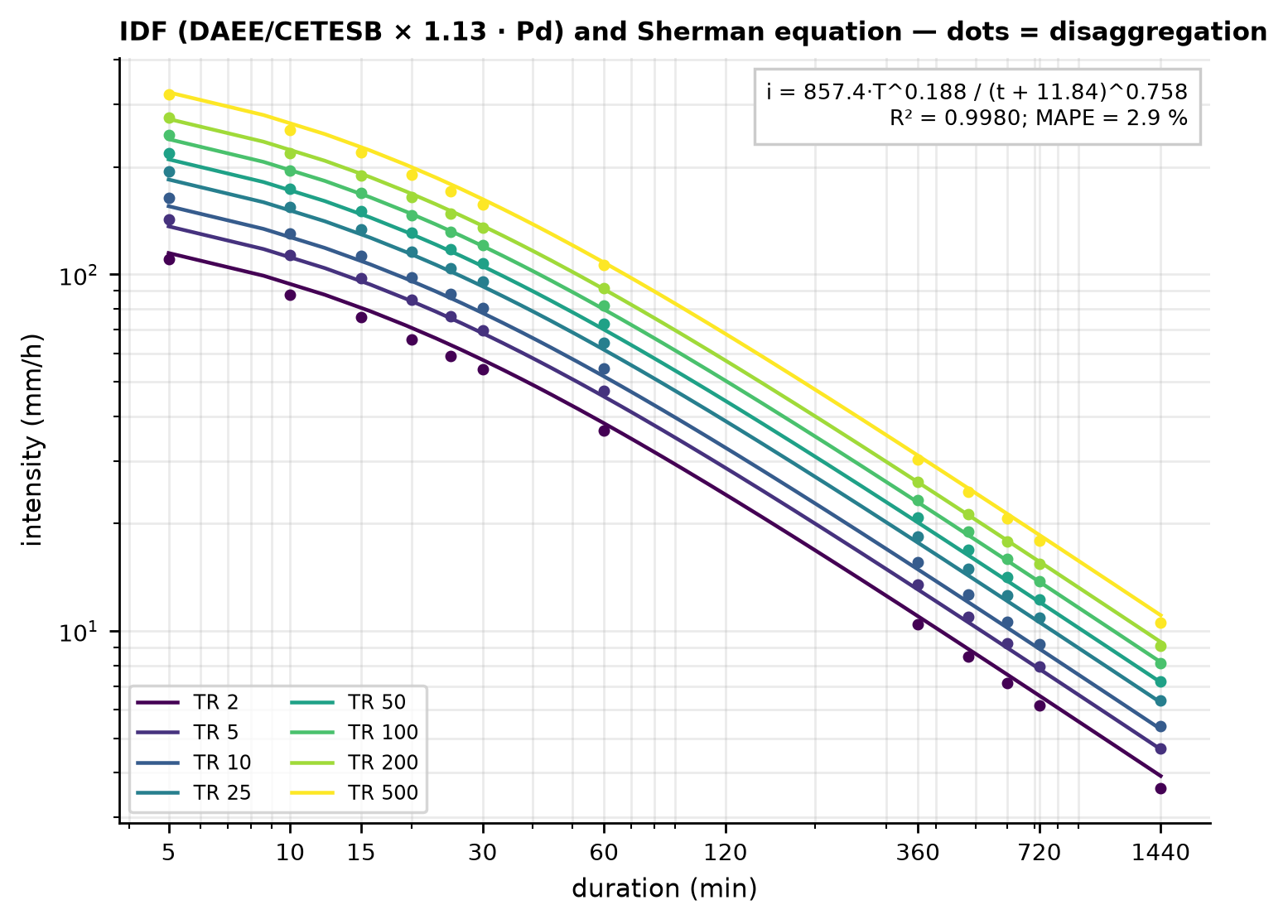
- intensity \(i = P/(d/60)\) and fit of the Sherman equation to the 96 points (8 return periods × 12 durations):
\[ i(t, T) = \frac{K\,T^{a}}{(t + b)^{c}} \quad [\text{mm/h}; t \text{ in min}; T \text{ in years}]. \]
| T (years) | 5 min | 10 min | 15 min | 30 min | 60 min | 360 min | 720 min | 1440 min |
|---|---|---|---|---|---|---|---|---|
| 2 | 110.4 | 87.7 | 75.8 | 54.1 | 36.6 | 10.4 | 6.2 | 3.6 |
| 5 | 142.4 | 113.1 | 97.7 | 69.8 | 47.2 | 13.5 | 8.0 | 4.7 |
| 10 | 164.3 | 130.5 | 112.8 | 80.6 | 54.4 | 15.6 | 9.2 | 5.4 |
| 25 | 194.5 | 154.5 | 133.5 | 95.3 | 64.4 | 18.4 | 10.9 | 6.4 |
| 50 | 219.3 | 174.2 | 150.5 | 107.5 | 72.6 | 20.8 | 12.3 | 7.2 |
| 100 | 246.4 | 195.7 | 169.1 | 120.8 | 81.6 | 23.3 | 13.8 | 8.1 |
| 200 | 276.1 | 219.3 | 189.5 | 135.4 | 91.5 | 26.1 | 15.4 | 9.1 |
| 500 | 320.1 | 254.2 | 219.7 | 156.9 | 106.0 | 30.3 | 17.9 | 10.5 |
The Sherman equation fitted to these 96 points is i = 857.44·T^0.1880/(t + 11.845)^0.7581 (mm/h; t in min; T in years), with R² = 0.9980, RMSE = 3.39 mm/h, and MAPE = 2.86%.
WarningLimitation
An IDF derived from daily rainfall with national disaggregation ratios does not replace an IDF from recording-gauge records. In 2011 the city’s automatic stations measured peaks of 40–63 mm/h (Table 6.1); the IDF gives 81.6 mm/h for 1 h at T = 100 years — consistent in order of magnitude, but without local validation of the sub-daily ratios.
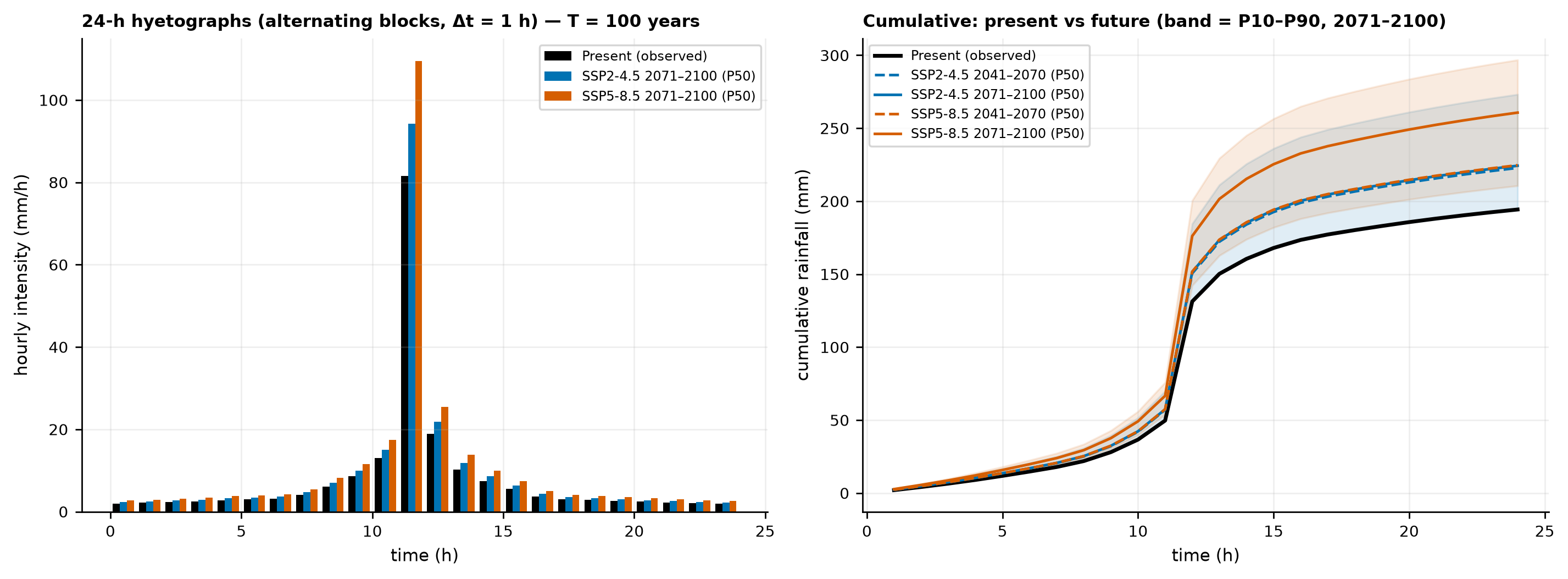
6.5.5 Design hyetograph by the alternating block method
TRIGRS needs rainfall as an intensity per period (m/s). The alternating block method (Chow et al., 1988, §14.4) builds a hyetograph that contains, around the peak, the IDF depths for all durations:
- choose the duration (24 h) and the time step (Δt = 1 h → 24 blocks);
- compute the cumulative depth \(P_k = P(k\,\Delta t)\) for k = 1…24 — here with the DAEE/CETESB relation interpolated in log–log space between the nodes (exact at 1, 6, 8, 10, 12, and 24 h, so that the total is exactly P24h);
- compute the increments \(\Delta P_k = P_k - P_{k-1}\) and sort them from largest to smallest;
- place the largest one in the central block (the 12th) and the following ones alternately to the right and to the left;
- convert to intensity: \(i\,[\text{m/s}] = \Delta P\,[\text{mm}] / (1000 \cdot 3600)\).
For T = 100 years: P24h = 194.3 mm; the central block (11–12 h) receives P(1 h) = 0.42 × 194.3 = 81.6 mm; the second largest increment, P(2 h) − P(1 h) = 18.9 mm, goes to 12–13 h, and so on (Table 6.15). The 200 hyetographs (8 return periods × 25 combinations: present + 4 SSPs × 2 horizons × 3 statistics) are in chuva/hietogramas_projeto.csv (columns cenario, horizonte, estatistica, tr, passo, t_ini_h, t_fim_h, mm, mm_h: scenario, horizon, statistic, return period, step, start and end times, depth, and intensity). With the Sherman equation instead of the DAEE/CETESB interpolation, the peak for T = 100 years would be 79.8 mm/h and the total 196.1 mm (+0.9%).
| Step | Hour | Present (mm) | Present (m/s) | SSP5-8.5 2071–2100 P50 (mm) | SSP5-8.5 (m/s) |
|---|---|---|---|---|---|
| 1 | 0–1 | 1.99 | 5.541e-07 | 2.68 | 7.434e-07 |
| 2 | 1–2 | 2.14 | 5.950e-07 | 2.87 | 7.983e-07 |
| 3 | 2–3 | 2.32 | 6.437e-07 | 3.11 | 8.636e-07 |
| 4 | 3–4 | 2.53 | 7.026e-07 | 3.39 | 9.427e-07 |
| 5 | 4–5 | 2.79 | 7.757e-07 | 3.75 | 1.041e-06 |
| 6 | 5–6 | 2.95 | 8.194e-07 | 3.96 | 1.099e-06 |
| 7 | 6–7 | 3.13 | 8.691e-07 | 4.20 | 1.166e-06 |
| 8 | 7–8 | 4.05 | 1.126e-06 | 5.44 | 1.511e-06 |
| 9 | 8–9 | 6.13 | 1.703e-06 | 8.23 | 2.285e-06 |
| 10 | 9–10 | 8.60 | 2.388e-06 | 11.54 | 3.204e-06 |
| 11 | 10–11 | 13.04 | 3.623e-06 | 17.50 | 4.860e-06 |
| 12 | 11–12 | 81.61 | 2.267e-05 | 109.49 | 3.041e-05 |
| 13 | 12–13 | 18.92 | 5.256e-06 | 25.38 | 7.051e-06 |
| 14 | 13–14 | 10.27 | 2.852e-06 | 13.77 | 3.826e-06 |
| 15 | 14–15 | 7.47 | 2.074e-06 | 10.02 | 2.783e-06 |
| 16 | 15–16 | 5.53 | 1.535e-06 | 7.42 | 2.060e-06 |
| 17 | 16–17 | 3.72 | 1.033e-06 | 4.99 | 1.386e-06 |
| 18 | 17–18 | 3.02 | 8.392e-07 | 4.05 | 1.126e-06 |
| 19 | 18–19 | 2.81 | 7.800e-07 | 3.77 | 1.047e-06 |
| 20 | 19–20 | 2.65 | 7.371e-07 | 3.56 | 9.889e-07 |
| 21 | 20–21 | 2.42 | 6.717e-07 | 3.24 | 9.011e-07 |
| 22 | 21–22 | 2.23 | 6.182e-07 | 2.99 | 8.294e-07 |
| 23 | 22–23 | 2.07 | 5.737e-07 | 2.77 | 7.697e-07 |
| 24 | 23–24 | 1.93 | 5.359e-07 | 2.59 | 7.190e-07 |
| Σ | 0–24 | 194.3 | — | 260.7 | — |
03_idf_hietogramas_clima.py (excerpt) — IDF and hyetograph
from trigrs_mapper.hydro.idf import tabela_idf, ajustar_sherman
from trigrs_mapper.hydro.hietograma import altura_duracao_daee_cetesb, hietograma_blocos_alternados

pd_tr = {2: 77.04, 5: 99.38, 10: 114.68, 25: 135.75, 50: 153.06, 100: 171.95, 200: 192.71, 500: 223.42}
tab = tabela_idf(pd_tr, metodo="daee_cetesb", fator_24h=1.13)    # 8 return periods × 12 durations
sherman = ajustar_sherman(tab)                                     # K, a, b, c, R², RMSE, MAPE

p24 = 1.13 * pd_tr[100]
h = hietograma_blocos_alternados(altura_duracao_daee_cetesb(p24), duracao_minutes=1440.0, dt_minutes=60.0)
print(h.total_mm, h.intensidade_mm_h.max(), h.intensidade_m_s.max())   # 194.3 mm; 81.6 mm/h; 2.27e-5 m/s
6.5.6 Effective rainfall (SCS-CN) and design hydrograph
6.5.6.1 Curve Number
The first source is BHAE 2022 in the DPM database (skill dpm-bhae-postgis; a drainage-area base derived from ANA’s Otto-coded hydrography, with ANA’s 2022 Curve Number product): the point falls in the 9.58 km² BHAE drainage area (Otto basin code cobacia 778483), whose 2022 CN from the ANA product (AMC II) has a mean of 74.6 and a median of 77 (Table 6.17). This area is ~85 times larger than the watershed and includes urban neighborhoods and forested slopes; for this reason the CN was checked against the land use and the hydrologic soil group of the watershed itself, with the TR-55 table (USDA-SCS, 1986) and group C for the Cambissolo Háplico (Sartori et al., 2005).
| Source | Class | TR-55 cover type | Watershed fraction (%) | CN (group C) | CN (group D) |
|---|---|---|---|---|---|
| MapBiomas 2025 | Rocky Outcrop | impervious | 47.2 | 98 | 98 |
| MapBiomas 2025 | Forest Formation | woods, good condition | 29.1 | 70 | 77 |
| MapBiomas 2025 | Pasture | pasture/grassland, fair | 17.3 | 79 | 84 |
| MapBiomas 2025 | Grassland | pasture/grassland, fair | 5.5 | 79 | 84 |
| MapBiomas 2025 | Mosaic of Uses | woods + pasture, fair | 0.8 | 76 | 82 |
| MapBiomas 2025 | Area-weighted mean CN | — | 100 | 85.3 | 88.6 |
| MapBiomas 2015 | Rocky Outcrop | impervious | 44.1 | 98 | 98 |
| MapBiomas 2015 | Pasture | pasture/grassland, fair | 19.7 | 79 | 84 |
| MapBiomas 2015 | Mosaic of Uses | woods + pasture, fair | 18.9 | 76 | 82 |
| MapBiomas 2015 | Forest Formation | woods, good condition | 11.8 | 70 | 77 |
| MapBiomas 2015 | Grassland | pasture/grassland, fair | 5.5 | 79 | 84 |
| MapBiomas 2015 | Area-weighted mean CN | — | 100 | 85.7 | 89.0 |
| GLAD 2010 | short vegetation (GLAD 0-24) | pasture/grassland, fair | 52.0 | 79 | 84 |
| GLAD 2010 | tree cover (GLAD 25-48) | woods, good condition | 48.0 | 70 | 77 |
| GLAD 2010 | Area-weighted mean CN | — | 100 | 74.7 | 80.6 |
bhae.bhae_cn2022) and adopted CN.
| Quantity | Value |
|---|---|
| BHAE drainage area (cobacia) | 778483 — 9.58 km² (local area) |
| ANA CN2: mean / median / min. / max. / std. dev. | 74.6 / 77 / 65 / 98 / 9.7 |
| Global CN (AMC I / II / III, mean) | 66.1 / 81.9 / 92.0 |
| Adopted CN (2025 land use × group C): AMC I / II / III | 70.9 / 85.3 / 93.0 |
| Runoff for T = 100 years (P24h; mean CN × class by class) | 150.1 mm × 150.8 mm |
The adopted CN is 85.3 (AMC II), from MapBiomas 2025 (current state, appropriate for design) with group C. It is higher than the BHAE value because 47% of the watershed is rock outcrop (CN 98). GLAD 2010 does not separate rock (it classifies the scarp as short vegetation) and would give 74.7 — which is why it is not used here. The wet antecedent moisture condition (AMC III), typical of a rainy summer such as that of 2010–2011, gives
\[ CN(III) = \frac{23\,CN(II)}{10 + 0.13\,CN(II)} = 93.0. \]
The cumulative effective rainfall follows SCS-CN with \(I_a = 0.2\,S\):
\[ S = \frac{25400}{CN} - 254 = 43.8\ \text{mm}, \quad I_a = 8.8\ \text{mm}, \quad Q = \frac{(P - I_a)^2}{P - I_a + S}\ \ (P > I_a). \]
For T = 100 years (P24h = 194.3 mm): Q = 150.1 mm (C = 0.77) with the mean CN; computing the runoff class by class and weighting by area, 150.8 mm — averaging the CN is adequate here.
6.5.6.2 Triangular unit hydrograph and design hydrograph
The adopted time of concentration is the median of the three formulas in Table 6.6: Ven Te Chow, 9.49 min (Kirpich and Giandotti as sensitivity cases). The SCS triangular unit hydrograph (NRCS NEH-630, Chapter 16) is:
\[ t_{lag} = 0.6\,t_c = 5.69\ \text{min}; \quad t_p = \frac{\Delta t}{2} + t_{lag} = 6.19\ \text{min}; \quad t_b = 2.67\,t_p = 16.5\ \text{min}; \quad q_p = \frac{0.208\,A}{t_p} = 0.226\ \frac{\text{m}^3/\text{s}}{\text{mm}} \]
(A in km², \(t_p\) in hours). With such a fast watershed, the time step of the hydrograph must be small: we use Δt = 1 min (≤ 0.25 \(t_p\)) and a 24-h hyetograph with 1-min blocks, in which durations below 5 min (the limit of the DAEE/CETESB ratios) receive the constant 5-min intensity. The discrete convolution of the effective rainfall with the unit hydrograph (volume conservation checked: zero balance error, up to rounding) gives the design hydrograph (Figure 6.22).
| T | P24h (mm) | Pe AMC II (mm) | C = Pe/P | Qp AMC II (m³/s) | Qp AMC III | Qp tc Kirpich | Qp tc Giandotti | Time to peak (h) | Volume (m³) |
|---|---|---|---|---|---|---|---|---|---|
| 2 | 87.1 | 50.2 | 0.58 | 1.84 | 2.39 | 2.32 | 1.67 | 12.12 | 5,645 |
| 5 | 112.3 | 72.8 | 0.65 | 2.65 | 3.21 | 3.33 | 2.40 | 12.12 | 8,181 |
| 10 | 129.6 | 88.7 | 0.68 | 3.21 | 3.76 | 4.04 | 2.91 | 12.12 | 9,970 |
| 25 | 153.4 | 111.0 | 0.72 | 3.99 | 4.52 | 5.01 | 3.62 | 12.12 | 12,480 |
| 50 | 173.0 | 129.6 | 0.75 | 4.62 | 5.15 | 5.80 | 4.19 | 12.10 | 14,572 |
| 100 | 194.3 | 150.1 | 0.77 | 5.32 | 5.82 | 6.67 | 4.82 | 12.10 | 16,875 |
| 200 | 217.8 | 172.8 | 0.79 | 6.08 | 6.56 | 7.62 | 5.51 | 12.10 | 19,424 |
| 500 | 252.5 | 206.6 | 0.82 | 7.20 | 7.65 | 9.02 | 6.53 | 12.10 | 23,223 |
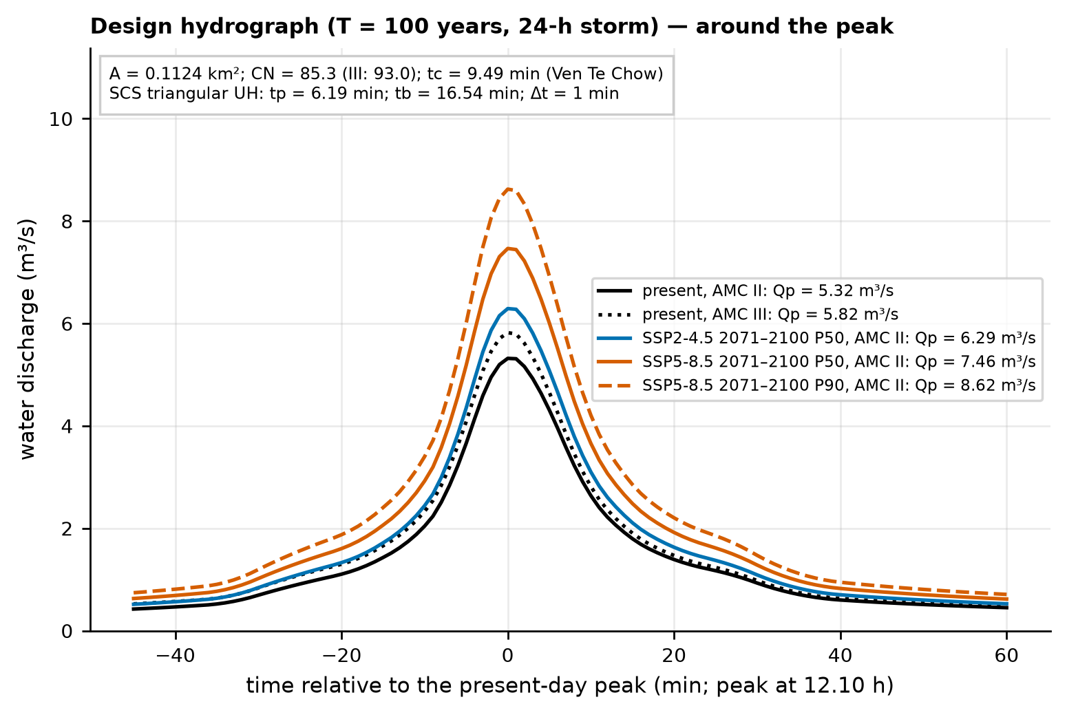
The clear-water peak discharge for T = 100 years is Qp = 5.32 m³/s (AMC II), 5.82 m³/s with AMC III, and 4.82–6.67 m³/s depending on tc — the uncertainty in tc weighs more than that in the antecedent moisture. The hydrographs of all scenarios are in chuva/hidrogramas_projeto.csv (AMC II) and chuva/hidrogramas_projeto_amc3.csv. The debris-flow peak discharge, which multiplies Qp by the factor \(K_q = C_*/(C_* - C_d)\), is computed in Section 6.7.
04_cn_hidrograma.py (excerpt) — SCS-CN and hydrograph
from trigrs_mapper.hydro.hidrograma import hidrograma_projeto
from trigrs_mapper.hydro.hietograma import hietograma_blocos_alternados
from trigrs_mapper.hydro.scs_cn import cn_condicao_umidade

cn2 = 85.3
cn3 = cn_condicao_umidade(cn2, "III")                     # 93.0
h = hietograma_blocos_alternados(altura_duracao_hidro(194.3), 1440.0, 1.0)   # 24 h, Δt = 1 min
hp = hidrograma_projeto(h, area_km2=0.1124, cn=cn2, tc_hours=9.49 / 60.0, lambda_ia=0.2)
print(hp.resumo()["qp_m3s"], hp.hu.tp_hours * 60.0)       # ≈ 5.32 m³/s; 6.19 min
6.5.7 Rainfall of the January 11–12, 2011 event (calibration input)
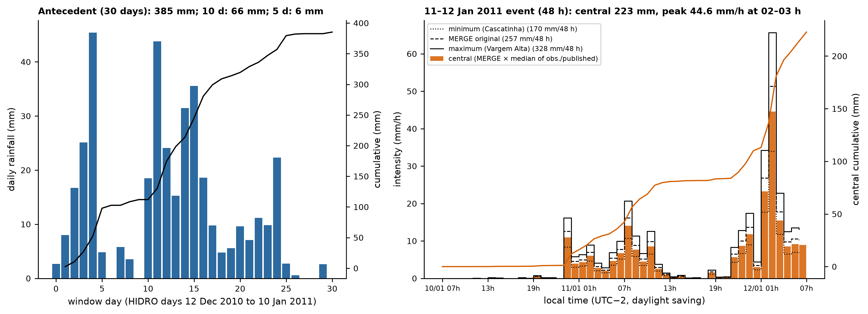
The TRIGRS calibration (Section 6.9) needs the hourly rainfall of the event and the antecedent rainfall. Since the hourly data of INMET and Cemaden (the National Center for Monitoring and Early Warning of Natural Disasters) are not accessible from the project’s server (decision D14), the hyetograph was reconstructed:
- hourly shape: MERGE/CPTEC-INPE (the rainfall product of the Center for Weather Forecasting and Climate Studies of the National Institute for Space Research: GPM IMERG merged with rain gauges; 0.1°; Rozante et al., 2010) in the cell that contains the point. The file of hour HH UTC was treated as the accumulation over the hour ending at HH (the peak at 05 UTC coincides with the 62.8 mm/h peak of the INMET automatic station; uncertainty of ±1 h);
- scaling: the 48-h total (HIDRO days January 11 and 12, i.e., from January 10, 07:00 to January 12, 07:00, local daylight-saving time, UTC−2) was set equal to the median of the 13 available totals — the 6 database rain gauges within 15 km (sum of January 11 + 12, to avoid the ±1-day shift of some observers) and 7 published values (Table 6.19); the minimum, the maximum, and MERGE without rescaling are kept as uncertainty scenarios;
- antecedent rainfall: 30 HIDRO days (December 12, 2010 to January 10, 2011) in daily steps, from the Xavier/BR-DWGD grid (Brazilian Daily Weather Gridded Data; Xavier et al., 2022; cell ~1.5 km away) extracted from the DPM database.
| Source | Dist. (km) | Jan 12 (mm) | Jan 11+12 or published (mm) |
|---|---|---|---|
| Vargem Grande | 4.1 | 183.5 | 197.2 |
| Cascatinha do Cônego | 9.4 | 109.3 | 170.0 |
| Fazenda Mendes | 12.7 | 225.4 | 325.9 |
| Teodoro de Oliveira | 13.1 | 34.6 | 147.0 |
| São Lourenço | 13.2 | 164.5 | 191.6 |
| Vargem Alta | 15.0 | 271.5 | 328.3 |
| Dourado et al. (2012) — INEA Olaria | — | — | 241.8 (24 h) |
| Dourado et al. (2012) — INEA Sítio Santa Paula | — | — | 240.0 (24 h (Jan 12)) |
| Dourado et al. (2012) — INEA Ypu | — | — | 222.8 (24 h) |
| Dourado et al. (2012) — INEA Nova Friburgo | — | — | 182.0 (24 h) |
| Climanálise (2011) — INMET Nova Friburgo | — | — | 166.0 (Jan 11–12) |
| Cabral et al. (2023) — Nova Friburgo (Rio Grande) | — | — | 249.0 (24 h) |
| Marc et al. (2018) — event rainfall over the landslide area | — | — | 280.0 (~36 h) |
chuva/evento_hietograma.csv; all of them are in evento_hietograma_cenarios.csv.
| Scaling scenario | Factor | 48 h (mm) | HIDRO day Jan 12 (mm) | Peak (mm/h) | Max. I3 (mm/h) | 30 d + 48 h window (mm) |
|---|---|---|---|---|---|---|
| minimum (Cascatinha do Cônego) | 0.662 | 170.0 | 137.6 | 34.0 | 21.2 | 555.3 |
| IDW of the rain gauges ≤ 15 km | 0.800 | 205.3 | 166.2 | 41.1 | 25.6 | 590.6 |
| central (median) | 0.868 | 222.8 | 180.3 | 44.6 | 27.7 | 608.1 |
| MERGE without rescaling | 1.000 | 256.8 | 207.8 | 51.3 | 32.0 | 642.0 |
| maximum (Vargem Alta) | 1.279 | 328.3 | 265.7 | 65.7 | 40.9 | 713.6 |
| Series | 5 days (mm) | 10 days (mm) | 15 days (mm) | 30 days (mm) |
|---|---|---|---|---|
| Xavier (cell 11600313) | 5.9 | 65.9 | 140.2 | 385.3 |
| Cascatinha do Cônego | 0.9 | 40.5 | 78.8 | 257.4 |
| Vargem Grande | 6.7 | 56.7 | 124.9 | 388.9 |
| Fazenda Mendes | 3.1 | 69.8 | 95.1 | 416.7 |
With the 30-day Xavier ETo (113.4 mm), the gross initial infiltration rate rizero is 1.49 × 10⁻⁷ m/s, the net rate 1.05 × 10⁻⁷ m/s, and the suggested rate 5.0 × 10⁻⁸ m/s (the cap of the recommended range, explained below).
The central scenario has 222.8 mm in 48 h and a peak of 44.6 mm/h between 02:00 and 03:00 on January 12 (local time), preceded by 385 mm in 30 days. The last 5 days before the event were almost dry (5.9 mm), which shows why the 30-day rainfall — and not that of a few days — controls the initial water table. The mean net 30-day rate (\((P_{30} - ETo_{30})/30\ \text{days}\) = 1.05 × 10⁻⁷ m/s) exceeds the 5 × 10⁻⁸ m/s cap recommended for rizero in the parameter step; the suggested value is the cap, and the very wet antecedent condition also enters through the initial water-table scenarios (decision D6).
6.6 Climate change
6.6.1 Method
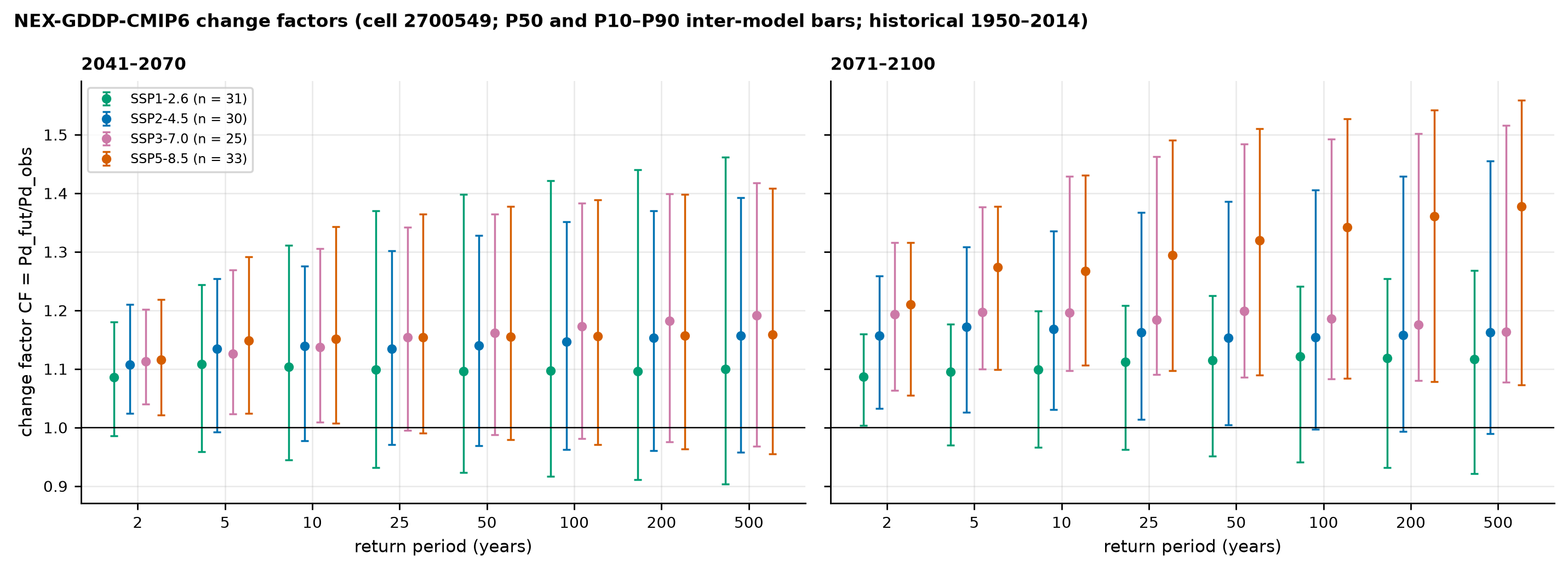
The method is that of the IDF-MC Portal (SEDEC/MIDR; data release 2026.08.002), reproduced by the project with a maximum relative difference of 1.6 × 10⁻⁷ from the public API (07_mudanca_climatica.md):
- for each NEX-GDDP-CMIP6 model (Thrasher et al., 2022; 0.25°), a Gumbel distribution is fitted by moments to the annual maxima of daily rainfall in the model’s own historical window (1950–2014) and in the future window (2041–2070 or 2071–2100);
- the model’s change factor is the ratio of the quantiles with the same return period, \(FC_m(T) = x_{T,\text{fut}}/x_{T,\text{hist}}\) — the model bias appears in both the numerator and the denominator and cancels out (the absolute values of the models are never used);
- the ensemble is summarized by the P10, P50, and P90 percentiles across models (inter-model spread, not a confidence interval; the SSPs have no probabilities);
- the future rainfall is \(P_{d,\text{fut}}(T) = FC(T) \cdot P_d(T)\), applied to the 1-day rainfall before the conversion to 24 h and the disaggregation: the future IDF and hyetographs are the present ones multiplied by the FC of each return period.
The cell of the point is 2700549 (center −42.625; −22.375), the same as that of the main Nova Friburgo point in the IDF-MC; the final point lies ~1 km from the northern edge of the cell. There are 31, 30, 25, and 33 models in SSP1-2.6, SSP2-4.5, SSP3-7.0, and SSP5-8.5.
6.6.2 Factors, future rainfall, and equivalent return period
| Scenario | Horizon | Models | % with FC > 1 | FC(100) P50 [P10–P90] | Pd100 (mm) | Pd200 (mm) | Equivalent T of today’s 100-year rainfall (years) |
|---|---|---|---|---|---|---|---|
| SSP1-2.6 | 2041–2070 | 31 | 74 | 1.10 [0.92–1.42] | 189 [158–244] | 211 [175–278] | 58 [17–175] |
| SSP1-2.6 | 2071–2100 | 31 | 77 | 1.12 [0.94–1.24] | 193 [162–213] | 216 [180–242] | 52 [32–150] |
| SSP2-4.5 | 2041–2070 | 30 | 77 | 1.15 [0.96–1.35] | 197 [165–232] | 222 [185–264] | 46 [22–127] |
| SSP2-4.5 | 2071–2100 | 30 | 87 | 1.15 [1.00–1.41] | 198 [171–242] | 223 [191–275] | 43 [17–102] |
| SSP3-7.0 | 2041–2070 | 25 | 84 | 1.17 [0.98–1.38] | 202 [169–238] | 228 [188–270] | 42 [19–113] |
| SSP3-7.0 | 2071–2100 | 25 | 96 | 1.19 [1.08–1.49] | 204 [186–257] | 226 [208–289] | 35 [12–61] |
| SSP5-8.5 | 2041–2070 | 33 | 88 | 1.16 [0.97–1.39] | 199 [167–239] | 223 [186–269] | 43 [17–124] |
| SSP5-8.5 | 2071–2100 | 33 | 94 | 1.34 [1.08–1.53] | 231 [186–263] | 262 [208–297] | 23 [12–60] |
Present: Pd100 = 172.0 mm; Pd200 = 192.7 mm.
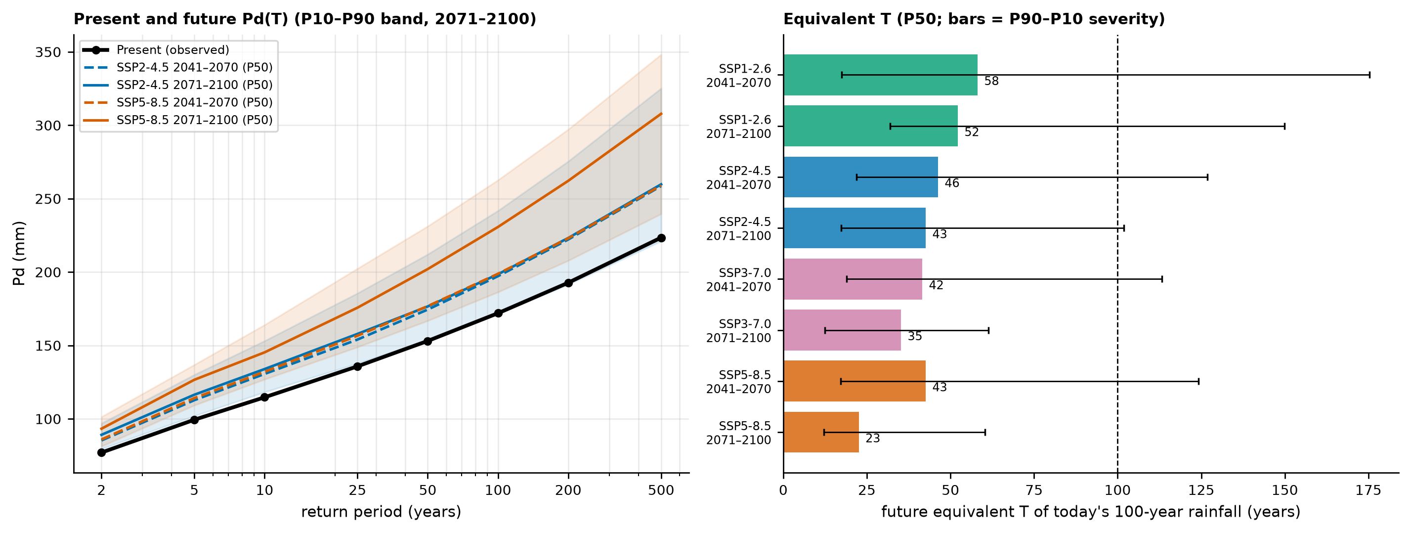
Reading:
- the ensemble median indicates an increase in all scenarios and horizons; at the end of the century, under SSP5-8.5, 94% of the models project an increase, and the 100-year rainfall goes from 172 to 231 mm [186–263];
- under SSP2-4.5 (end of the century) the median increase is 15% (198 mm [171–242]); in mid-century the SSPs do not yet separate (FC from 1.10 to 1.17);
- the rainfall that today has a 100-year return period would have a return period of ~23 years (SSP5-8.5, 2071–2100) or ~43 years (SSP2-4.5, 2071–2100). The equivalent return period was computed model by model, by solving \(FC_m(T)\,x(T) = x(100)\) with the adopted GLO distribution; with the manual’s Gumbel the change would be larger (15.3 years; 07_mudanca_climatica.md), because the GLO tail is heavier;
- the inter-model spread (P90 − P10 of 0.3 to 0.5 in the FC) is of the same order as the signal itself: always use the range.
The future hyetographs are in Figure 6.21 and Table 6.15 (SSP5-8.5 2071–2100 P50: 260.7 mm in 24 h and 109.5 mm in the peak block for T = 100 years). The Sherman parameters of each scenario are in chuva/clima.json.
WarningLimitations of the factors
- the cell covers ~700 km² and the watershed 0.11 km²: the FC of the areal mean rainfall is transferred to point rainfall;
- the Gumbel form is imposed in both windows, and the FC for T ≥ 100 years is an extrapolation from the 30-year future window;
- only the 1-day rainfall changes — the sub-daily ratios are kept, which may underestimate the increase in short-duration rainfall (Fowler et al., 2021);
- the change in multi-day antecedent rainfall is not represented.
6.7 The traditional GIDES/JICA method
The manual’s design volume is the smaller of what the watershed can generate (Vdy1) and what the design rainfall can transport (Vdy2), with a minimum of 1,000 m³, plus the woody debris (Vwy). Here it is computed with the data of the watershed and with trigrs_mapper.sabo, tested against Appendix A.
6.7.1 Vdy11 — erodible material in the channel bed (order ≥ 1)
\[ V_{dy11} = \sum A_{dy11}\,L_{dy11}, \qquad A_{dy11} = B_d \cdot D_e. \]
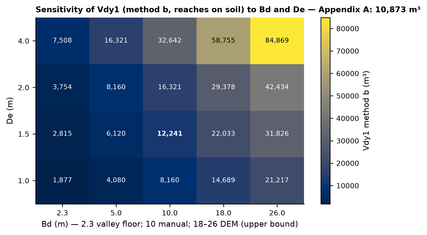
The manual requires \(B_d\) (mean width of the bed where erosion is expected) and \(D_e\) (mean erodible depth) from the field. Without fieldwork, we adopted:
- \(B_d\) = 10 m: the width used by Appendix A itself (Table 5.2). The DEM gives 14–26 m (median of 18 m; an upper bound, below the resolution; Table 6.3) and the manual records a 2.3 m valley floor in the erosion reach — both extremes enter the sensitivity analysis;
- \(D_e\) = 1.5 m: the median of the mean erosion depths observed in a reference Japanese disaster (NILIM, 2016a, Fig. 4(2): 50% ≤ 1.5 m, ~80% ≤ 2.0 m, maximum of 4.0 m; values read from the chart), consistent with the 0.5–2.0 m failures of Nova Friburgo (Marques et al., 2017);
- reaches over rock outcrop (MapBiomas 2025) have no erodible material: Appendix A also disregarded the reach between sections 6 and 7, on rock, and the soil over the rock at the headwater.
| Reach | L (m) | % on rock (MB 2025) | % on rock (MB 2015) | L on soil (m) | Volume Bd·De·L, soil (m³) | Volume, all reaches (m³) |
|---|---|---|---|---|---|---|
| order 1 | 207.3 | 41.6 | 6.7 | 121.0 | 1,815 | 3,110 |
| order 2 | 271.4 | 0.0 | 0.0 | 271.4 | 4,071 | 4,071 |
| order 0 (headwater) | 922.0 | 66.9 | 66.1 | 305.3 | 4,580 | 13,830 |
| order 0 (lateral) | 118.3 | 0.0 | 0.0 | 118.3 | 1,774 | 1,774 |
| Total order ≥ 1 (Vdy11) | 478.7 | — | — | 392.4 | 5,886 | 7,180 |
| Total order 0 (Vdy12, method b) | 1,040.3 | — | — | 423.6 | 6,355 | 15,604 |
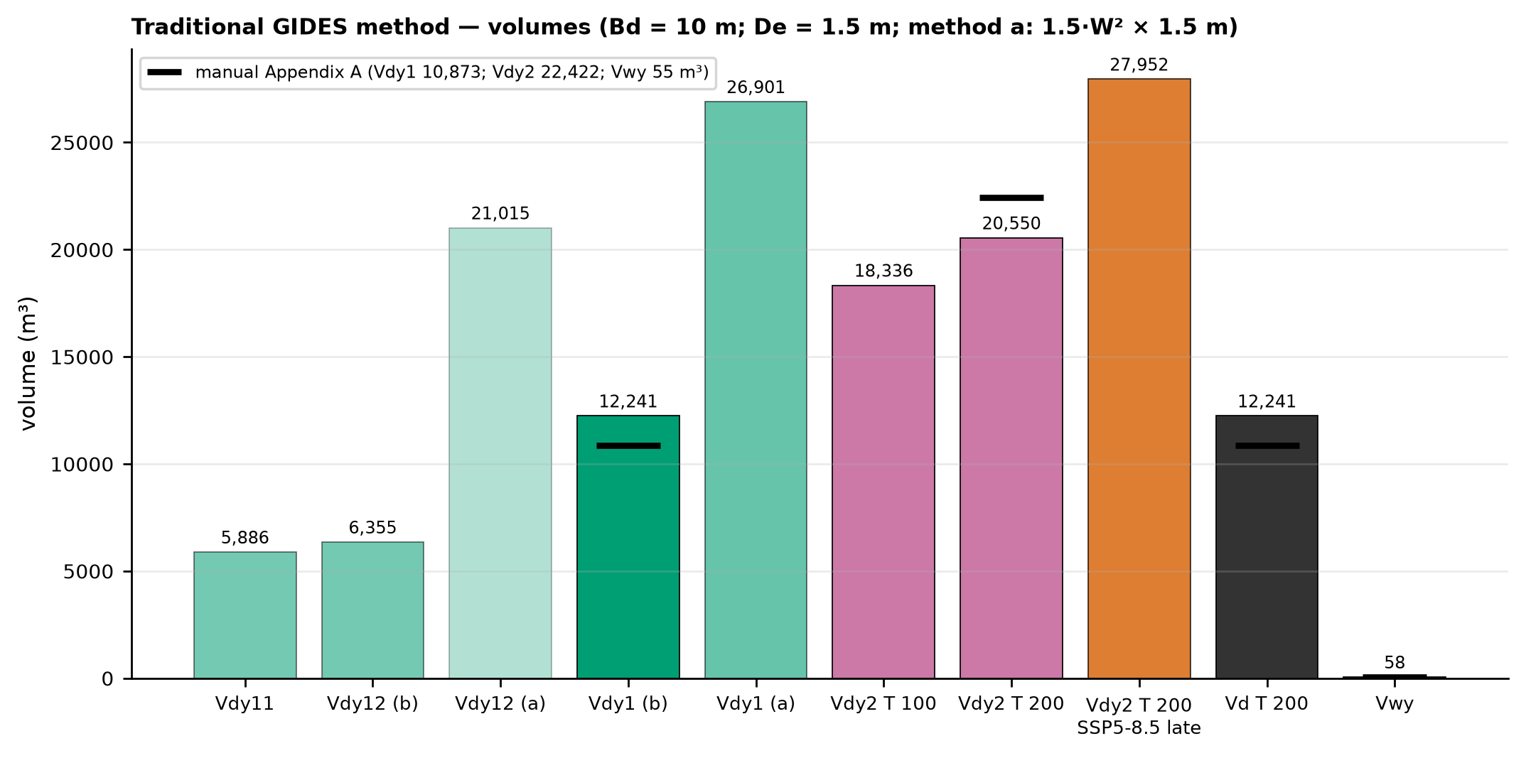
Result: Vdy11 = 10 × 1.5 × 392.4 = 5,886 m³ (7,180 m³ without excluding the rock). The first-order channels that descend the scarp face are 42% over rock in MapBiomas 2025 and only 7% in the 2015 map — a classification difference in the 30 m pixels at the foot of the scarp that changes Vdy11 by ~1,100 m³.
6.7.2 Vdy12 — hillslope material (order zero)
Method “b” (without a failure map): the same \(B_d \cdot D_e\) applied to the zero-order thalwegs (the manual says to estimate it “analogously”): Vdy12(b) = 15 × 423.6 = 6,355 m³ (15,604 m³ without excluding the rock — 67% of the headwater thalwegs lie on the scarp rock).
Method “a” (with a failure map): the 2011 scars are the best record of what fails in this watershed. Since the inventory lumps failure, track, and deposit into the same polygon, the failure area was approximated in two ways (02_inventarios.md): the upper third of each polygon by elevation, and the area \(A_s = 1.5\,W^2\) in the highest cells (Marc et al., 2018), always clipped to the watershed; the thickness ranges from 1 to 2 m.
| Approximate failure zone | Scars | Area in the watershed (m²) | h = 1.0 m | h = 1.5 m | h = 2.0 m |
|---|---|---|---|---|---|
| upper third by elevation | 5 | 20,492 | 20,492 | 30,738 | 40,984 |
| 1.5·W² (Marc et al., 2018) | 5 | 14,010 | 14,010 | 21,015 | 28,020 |
We adopted as the central value of method “a” the \(1.5\,W^2\) area with 1.5 m: Vdy12(a) = 21,015 m³ (range of 14,010 to 40,984 m³). For comparison, the global empirical volume–area relationship of Larsen et al. (2010), applied to the same five complete scars, gives ~49,000 m³ — the same order of magnitude.
6.7.3 Vdy1, Kf2, and Cd
\[ V_{dy1} = V_{dy11} + V_{dy12}: \qquad V_{dy1}^{(b)} = 5{,}886 + 6{,}355 = 12{,}241\ \text{m}^3; \qquad V_{dy1}^{(a)} = 5{,}886 + 21{,}015 = 26{,}901\ \text{m}^3. \]
Method “b” gives 12,241 m³, 13% above the manual’s field-based Vdy1 (10,873 m³) — good agreement for a calculation based only on open data, but one that depends on \(B_d \cdot D_e\): Figure 6.26 shows that Vdy1 ranges from ~1,900 to ~85,000 m³ over the plausible range of the two parameters; the manual’s value corresponds to \(B_d \cdot D_e \approx 13\) m².
The correction factor \(K_{f2}\) (Fig. 14 of the manual) and the concentration \(C_d\) (Takahashi; Annex 4 of the manual):
\[ K_{f2} = 0.05\,(\log_{10} A - 2)^2 + 0.05 = 0.05\,(\log_{10} 0.1124 - 2)^2 + 0.05 = 0.485 \quad (0.1 \le K_{f2} \le 0.5), \]
\[ C_d = \frac{\rho\,\tan\theta}{(\sigma - \rho)(\tan\phi - \tan\theta)} = \frac{1200 \times \tan 16.7°}{1400\,(\tan 35° - \tan 16.7°)} = 0.64 \;\rightarrow\; 0.54, \]
with σ = 2,600 kg/m³, ρ = 1,200 kg/m³, φ = 35°, and θ = 16.7° (mean slope over the 200 m upstream of the point; NILIM, 2016a, §2.6.3); the value is capped at \(0.9\,C_* = 0.54\) (\(C_*\) = 0.6). Cd stays at 0.54 for any θ above ~15° (the manual used θ = 20°); with NILIM’s 10° minimum, Cd would drop to 0.30.
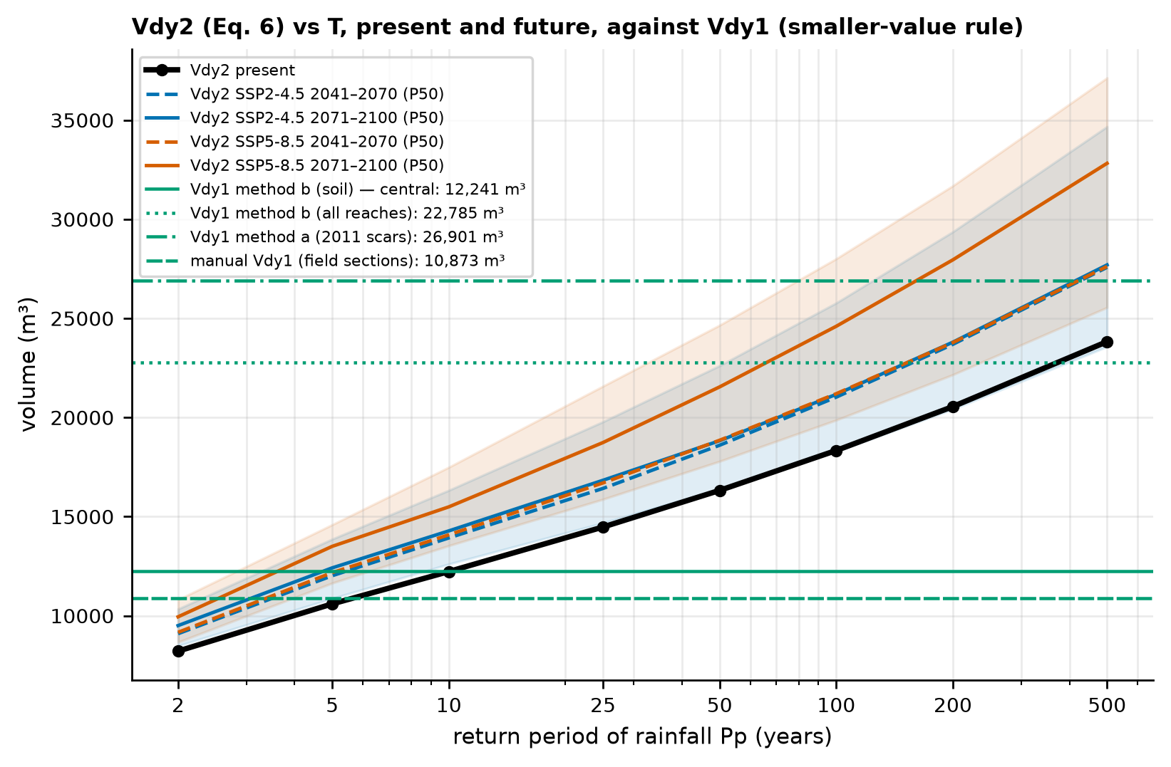
6.7.4 Vdy2 — volume transportable by the design rainfall
\[ V_{dy2} = \frac{10^3\,P_p\,A}{1 - K_v}\cdot\frac{C_d}{1 - C_d}\cdot K_{f2}, \qquad K_v = 0.4. \]
For T = 200 years (Pp = 192.7 mm): \(V_{dy2} = 10^3 \times 192.7 \times 0.1124 / 0.6 \times (0.54/0.46) \times 0.485 \approx\) 20,550 m³ (manual: 22,422 m³, with A = 0.12 km² and Kf2 = 0.5). Since Vdy2 is linear in Pp, climate change multiplies it by the FC.
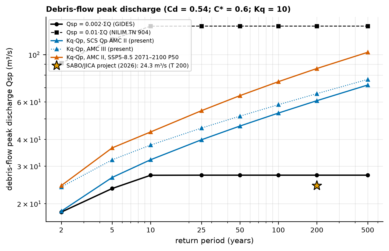
| T | Pp (mm) | Vdy2 (m³) | Governs | Vd (m³) | Total with woody debris (m³) | Qsp 0.002 (m³/s) | Qsp 0.01 (m³/s) | Water Qp (m³/s) | Kq·Qp (m³/s) |
|---|---|---|---|---|---|---|---|---|---|
| 2 | 77.0 | 8,215 | Vdy2 | 8,215 | 8,273 | 18.3 | 91.3 | 1.84 | 18.4 |
| 5 | 99.4 | 10,598 | Vdy2 | 10,598 | 10,656 | 23.6 | 117.8 | 2.65 | 26.5 |
| 10 | 114.7 | 12,229 | Vdy2 | 12,229 | 12,288 | 27.2 | 135.9 | 3.21 | 32.1 |
| 25 | 135.7 | 14,475 | Vdy1 | 12,241 | 12,299 | 27.2 | 136.0 | 3.99 | 39.9 |
| 50 | 153.1 | 16,322 | Vdy1 | 12,241 | 12,299 | 27.2 | 136.0 | 4.62 | 46.2 |
| 100 | 172.0 | 18,336 | Vdy1 | 12,241 | 12,299 | 27.2 | 136.0 | 5.32 | 53.2 |
| 200 | 192.7 | 20,550 | Vdy1 | 12,241 | 12,299 | 27.2 | 136.0 | 6.08 | 60.8 |
| 500 | 223.4 | 23,825 | Vdy1 | 12,241 | 12,299 | 27.2 | 136.0 | 7.20 | 72.0 |
| Scenario | Horizon | T | Pp P50 [P10–P90] (mm) | Vdy2 P50 [P10–P90] (m³) | Vd, method b (m³) | Vd with Vdy12 by method a (m³) | Kq·Qp P50 (m³/s) |
|---|---|---|---|---|---|---|---|
| SSP2-4.5 | 2041–2070 | 100 | 197.2 [165.5–232.3] | 21,027 [17,644–24,775] | 12,241 | 21,027 | 62.4 |
| SSP2-4.5 | 2041–2070 | 200 | 222.2 [185.0–264.1] | 23,691 [19,730–28,161] | 12,241 | 23,691 | 71.5 |
| SSP2-4.5 | 2071–2100 | 100 | 198.5 [171.4–241.8] | 21,166 [18,282–25,780] | 12,241 | 21,166 | 62.9 |
| SSP2-4.5 | 2071–2100 | 200 | 223.2 [191.4–275.4] | 23,800 [20,415–29,368] | 12,241 | 23,800 | 71.9 |
| SSP5-8.5 | 2041–2070 | 100 | 198.8 [167.0–238.8] | 21,200 [17,804–25,462] | 12,241 | 21,200 | 63.0 |
| SSP5-8.5 | 2041–2070 | 200 | 223.0 [185.7–269.4] | 23,779 [19,801–28,723] | 12,241 | 23,779 | 71.8 |
| SSP5-8.5 | 2071–2100 | 100 | 230.7 [186.3–262.7] | 24,601 [19,870–28,009] | 12,241 | 24,601 | 74.6 |
| SSP5-8.5 | 2071–2100 | 200 | 262.1 [207.8–297.2] | 27,952 [22,159–31,689] | 12,241 | 26,901 | 86.0 |
6.7.5 Woody debris (Vwy)
\[ V_{wy} = \frac{B_d\,L_{dy13}}{100}\sum V_{wy2}, \qquad V_{wy2} = \frac{\pi\,DAP^2}{4}\,H_w\,K_d. \]
With the visual survey of Appendix A (8 trees per 100 m², DAP (diameter at breast height) = 0.25 m, Hw = 6 m, Kd = 0.6 → Vwy2 = 0.177 m³ and ΣVwy2 = 1.414 m³/100 m²), Bd = 10 m, and \(L_{dy13}\) = the reach of the main thalweg under tree cover in GLAD 2010 (55.5% of 743.3 m = 412.6 m; the manual used 390 m): Vwy = 58 m³ (manual: 55 m³; 42 m³ with the MapBiomas 2025 forest). As in Appendix A, Kw = 1 (the SABO Project used Kw = 0.9).
6.7.6 Design volume (Vd) and debris-flow peak discharge (Qsp)
\[ V_d = \max\left[\min(V_{dy1}, V_{dy2}),\ 1{,}000\ \text{m}^3\right]; \qquad \Sigma Q = \frac{C_*\,V_d}{C_d}; \qquad Q_{sp} = 0.002\,\Sigma Q \ \text{(GIDES)}\ \text{or}\ 0.01\,\Sigma Q\ \text{(NILIM)}; \qquad Q_{sp} = K_q\,Q_p,\ K_q = \frac{C_*}{C_* - C_d}. \]
In the present climate, Vdy1 governs from T = 25 years upward: Vd = 12,241 m³ and a total volume with woody debris of 12,299 m³ (manual: 10,928 m³). With Vd = 12,241 m³: ΣQ = 0.6 × 12,241/0.54 = 13,601 m³ and Qsp = 27.2 m³/s (0.002·ΣQ; SABO Project/JICA: 24.3 m³/s), or 136 m³/s with the Japanese coefficient of 0.01. From the hydrograph, with \(K_q\) = 10 (because Cd = 0.54 is close to \(C_*\) = 0.6), Qsp = 10 × 5.32 = 53.2 m³/s for T = 100 years and 60.8 m³/s for T = 200 years.
NoteWhy do the discharges diverge so much?
The GIDES coefficient of 0.002 is 5 times smaller than the 0.01 of the Japanese standard (NILIM TN 904, Eq. 10) from which the relationship derives, with no justification in the manual; and \(K_q \cdot Q_p\) is very sensitive to Cd when Cd approaches \(C_*\). The manual’s hierarchy uses the empirical relationship as the primary estimate and \(K_q \cdot Q_p\) as a check. For design, report the envelope (27–136 m³/s for T = 200 years).
6.7.7 Comparison with Appendix A and what it teaches
| Quantity | Appendix A | This study |
|---|---|---|
| Watershed area (km²) | 0.075 (plan); 0.12 (in Vdy2) | 0.1124 |
| Kf2 | 0.477 computed; 0.5 adopted | 0.485 |
| θ (°) and Cd | 20°; 0.54 (limit 0.9·C*) | 16.7°; 0.54 (raw 0.64) |
| Pp, T = 200 years (mm) | 191 | 192.7 |
| Vdy1 (m³) | 10,873 (field cross-sections) | 12,241 (method b, reaches over soil) |
| Vdy2, T = 200 years (m³) | 22,422 | 20,550 |
| Smaller-value rule | Vdy1 governs | Vdy1 governs |
| Vwy (m³) | 55 | 58 |
| Total volume (m³) | 10,928 | 12,299 |
| Qsp = 0.002·ΣQ (m³/s) | 24.3 (SABO Project/JICA, 2026) | 27.2 |
Three lessons prepare the physical part of the study:
- The watershed is limited by sediment availability, as in the manual: for T ≥ 25 years, Vdy1 < Vdy2. Therefore, scaling up the rainfall does not change the design volume under the traditional method: under SSP5-8.5, at the end of the century, Vdy2 for T = 200 years rises from 20,550 to 27,952 m³ (+36%), but Vd remains 12,241 m³.
- Vdy12 is the weak link: by method “b” (length × cross-section) it is 6,355 m³; from the 2011 scars (method “a”), 14,010 to 40,984 m³. With method “a” the watershed becomes transport-limited and the design volume starts to respond to climate: for T = 100 years, from 18,336 m³ (present) to 21,166 m³ (SSP2-4.5) and 24,601 m³ (SSP5-8.5) at the end of the century.
- This is exactly the gap that TRIGRS fills: instead of an assumed length × cross-section, it estimates, for each design rainfall (present and future), which slopes fail and how thick the failed mass is — the physically based Vdy12 (Section 6.8 to Section 6.10).
06_gides.py (excerpt) — traditional method with trigrs_mapper.sabo
from trigrs_mapper.sabo import (TrechoErodivel, vdy1_m3, kf2, cd_takahashi, vdy2_m3, volume_projeto,
                                soma_q_m3, qsp_envelope, kq)

trechos = [TrechoErodivel(121.0, 10.0, 1.5, ordem=1), TrechoErodivel(271.4, 10.0, 1.5, ordem=2),
           TrechoErodivel(305.3, 10.0, 1.5, ordem=0), TrechoErodivel(118.3, 10.0, 1.5, ordem=0)]  # L over soil
v1 = vdy1_m3(trechos)                                   # Vdy11 ≈ 5,886; Vdy12 ≈ 6,355; Vdy1 ≈ 12,241 m³
cd = cd_takahashi(16.7).cd                              # 0.54 (raw 0.64)
v2 = vdy2_m3(192.71, 0.1124, cd, kf2(0.1124))           # ≈ 20,550 m³ (T = 200 years)
vp = volume_projeto(v1["vdy1_m3"], v2, 58.3)            # Vdy1 governs; total ≈ 12,299 m³
print(qsp_envelope(soma_q_m3(vp["volume_sedimentos_m3"], cd)), kq(cd))   # 27.2 and 136 m³/s; Kq = 10
6.8 TRIGRS modeling
The previous sections followed the empirical path of the GIDES manual. From here on we follow the physically based path proposed in Chapter 1 (Section 1.4.1): TRIGRS computes, in every grid cell and at every instant of the storm, the factor of safety \(FS(Z,t)\) and the critical depth \(Z_{cr}\) — first with the 2011 rainfall, to calibrate the model against the scars, and then with the design rainfalls of Section 6.5.5, in the present and future climates, to estimate the physically based Vdy12. The theory (infinite slope, transient infiltration, critical depth) is in Chapter 1, and the step-by-step walk-through of a run is in Chapters 4 and 5. What changes in a real watershed is the parameterization: instead of 100 synthetic cells with two zones, we have thousands of cells with properties derived from the datasets of Section 6.3, spatially variable soil thickness and initial water table, and a storm reconstructed from observations (Figure 6.30).
6.8.1 Model domains and grids
TRIGRS reads ESRI ASCII grids that must be congruent: the same extent, the same resolution, and the NODATA value (−9999) in the same positions in all of them, because the program only checks the cell count (Chapter 4). The project pipeline (trigrs_mapper.grids) prepares two domains:
- calibration window (
NF_calibracao, the same as in Section 6.1): 16,384 cells of 30 m (14.7 km²) on both faces of Morro Duas Pedras, where the 2011 scars used in the calibration lie; - watershed: the bounding rectangle of the reference-point watershed with a 300 m buffer and NODATA outside the mask — at 10 m (1,124 valid cells, 0.112 km²) for the final runs and at 30 m for the resolution comparison.
Why two resolutions? A run at 10 m costs about 9 times the same run at 30 m (decision D12), and the calibration requires 151 runs (Section 6.9.4). The search is carried out at 30 m, the native ANADEM resolution, and the calibrated multipliers are transferred to the 10 m watershed — a resampled DEM, which does not create information (D5) but draws the watershed outline and the D8 paths better. The price of this choice is measured in the sensitivity analysis, which compares the event on the watershed at 30 and at 10 m and checks the calibrated configuration on the window itself at 10 m (Section 6.9.7).
In each domain the pipeline writes the terrain grids — conditioned DEM (the same as in Section 6.4, used by TopoIndex), slope (Horn, 1981, computed on the raw DEM), D8 directions in the TopoIndex scheme (1 to 9, as in Chapter 4), contributing area, channels (A ≥ 1 ha, the threshold of Section 6.4), curvatures (Zevenbergen and Thorne, 1987), and topographic wetness index — and the cell-by-cell parameter grids described below: zones, zmax, depthwt, and rizero.
6.8.2 Geotechnical units, land cover, and property zones
Each zone of tr_in.txt needs eight numbers: cohesion \(c\), friction angle \(\varphi'\), unit weight \(\gamma_s\), diffusivity \(D_0\), saturated hydraulic conductivity \(K_s\), saturated and residual water contents (\(\theta_s\), \(\theta_r\)), and the parameter \(\alpha\) of the unsaturated model (Chapter 4). The zones are built in three steps.
1. Geotechnical unit. Each cell receives the unit of the first rule it satisfies (Table 6.28). There is no slope rule for “rock”: even among the steepest cells of the regional window, most are not outcrop in MapBiomas, and a slope threshold is not supported by the data.
trigrs_mapper.params). In the watershed, the IBGE soil unit is a Cambisol (CXbd32, Figure 6.6), so the shallow soil comes only from the outcrop neighborhood, and there is no orthogneiss.
| Order | Unit | Rule | In Nova Friburgo |
|---|---|---|---|
| 1 | rock outcrop | MapBiomas class 29 in 2015 and in 2025 (persistent outcrop, so that a recent scar is not mistaken for rock) | the scarp of Morro Duas Pedras (Figure 6.11) |
| 2 | talus/alluvial deposit | Quaternary deposits of the SGB 1:100,000 map (Qca, Qt…) or valley floor: A ≥ 1 ha and slope < 10° (the GIDES deposition range) |
a few valley-floor cells |
| 3 | colluvium | concavity (plan curvature < 0) with A ≥ 0.25 ha — the zero-order thalwegs of Section 6.4 | the concave lines of the hillslopes |
| 4 | shallow soil over rock | immediate neighborhood (8 cells) of the outcrop — Litholic Neossolo (Leptosol), with a zmax cap of 0.5 m (Santos et al., 2018) — or an IBGE soil unit dominated by rock outcrop |
the strip around the scarp |
| 5 | mature residual soil | all remaining cells, split into granite × orthogneiss by the 1:100,000 map | the soil-mantled hillslopes, all on granite (Figure 6.8) |
2. Root cohesion by land cover. Roots reinforce the soil mainly in the top 30–50 cm (Marques et al., 2018; José, 2016), but the failures in the region occur at 1–2.5 m. Since TRIGRS uses a single cohesion per zone, constant with depth, the root contribution enters as a small effective cohesion on the failure plane, added to that of the soil: \(c = c' + C_r\). The central values by land-cover group are 2 kPa for forest (G1 — the increment measured by José (2016) in in situ shear tests in Nova Friburgo), 1.5 kPa for silviculture (G2), 0.5 kPa for herbaceous vegetation, pasture, and mosaic of uses (G3), and zero for annual cropland (G4) and the areas without roots (G0); those of G2 to G4 are estimates. The land cover is that of the time of each run: GLAD 2010 for the 2011 event (trees → G1; short vegetation → G3) and MapBiomas 2025 for the design runs (current condition).
3. Zones. Each (unit, lithology, land-cover group) combination present in the domain becomes a zone, numbered from 1 to N (TRIGRS requires contiguous numbers). The parameters of each zone start from the a priori values of Table 6.29 — a review of laboratory and field tests from the Rio de Janeiro Highlands and the Serra do Mar compiled for the project — and are modified by global multipliers, the same for all zones, which the calibration adjusts (Section 6.9.4):
\[ \begin{aligned} c &= c'_0\,m_c + C_r\,m_{Cr}, & \tan\varphi' &= m_{\tan\varphi}\,\tan\varphi'_0,\\ K_s &= K_{s0}\,m_{Ks}, & D_0 &= r_{D0}\,K_s,\\ \alpha &= \alpha_0\,m_\alpha, & \gamma_s &= \gamma_w\left[G_s\,(1-\theta_s) + \theta_s\right]. \end{aligned} \]
Calibrating multipliers, rather than each number, preserves the spatial pattern given by the maps (which unit is more cohesive or more permeable than another) and reduces the search to 10 dimensions. Diffusivity follows the rule \(D_0 = r_{D0}\,K_s\), with \(r_{D0}\) = 200 m a priori (Park et al., 2013). The unit weight is derived from \(\theta_s\) with a fixed \(G_s\): in unsaturated mode TRIGRS computes \(G_s = (\gamma_s/\gamma_w - \theta_s)/(1-\theta_s)\), and \(\gamma_s\)–\(\theta_s\) pairs chosen independently would give physically impossible grain densities.
data/interim/parametros/tabela_parametros.yaml and in the project report docs/pesquisa/04_parametros_trigrs.md.
| Unit | c′ (kPa) | φ′ (°) | γs (kN/m³) | Ks (m/s) | θs / θr | α (1/m) | Main sources |
|---|---|---|---|---|---|---|---|
| colluvium | 3 (0–10) | 34 (26–42) | 18.0 | 1 × 10⁻⁵ | 0.48 / 0.08 | 5 | José (2016); Listo et al. (2018) |
| mature residual soil | 5 (0.5–15) | 35 (21–48) | 17.8 | 1 × 10⁻⁵ | 0.50 / 0.10 | 7 | Oliveira (2013); Machado (2016); Esteves et al. (2024) |
| shallow soil over rock | 2 (0–8) | 37 (32–45) | 18.5 | 2 × 10⁻⁵ | 0.45 / 0.06 | 6 | estimate anchored on Oliveira (2013) and Avelar (2023) |
| talus/alluvial deposit | 1 (0–6) | 36 (29–42) | 19.6 | 5 × 10⁻⁵ | 0.38 / 0.05 | 8 | estimate anchored on Avelar (2023) |
| rock outcrop | 100 | 45 | 26.0 | 1 × 10⁻⁹ | 0.05 / 0.01 | −1 | numerical convention (α < 0: saturated model) |
Table 6.30 shows the zones actually present in the 10 m watershed (MapBiomas 2025 land cover, that of the design runs), already with the calibrated multipliers and with the same numbering as the design tr_in.txt annotated in Section 6.8.6, and Figure 6.31 shows where they are. The outcrop stays in the model even though it does not fail: it generates surface runoff, which TopoIndex routes to the hillslopes and valleys downslope.
tr_in.txt) with the calibrated multipliers (full calibration, sample lhs_0019: mc = 0.92, mtanφ = 1.04, mKs = 0.70, rD0 = 39 m, mα = 0.57, mCr = 1.42). c′ = c′0·mc and cr = Cr·mCr (total cohesion c = c′ + cr); tan φ′ = mtanφ·tan φ′0; Ks = Ks0·mKs; D0 = rD0·Ks; α = α0·mα; γs derived from θs and Gs. The rock outcrop is the conventional, uncalibrated zone (α < 0: saturated infiltration). The event run uses the event land cover and a different numbering (event zone table).
| Zone · unit (lithology) · land cover | c′ + cr (kPa) | φ′ (°) | γs (kN/m³) | Ks (m/s) | D0 (m²/s) | θs / θr | α (1/m) | Area (%) |
|---|---|---|---|---|---|---|---|---|
| 1 · colluvium · G0 | 2.77 + 0.00 | 34.9 | 18.02 | 7.02 × 10⁻⁶ | 2.74 × 10⁻⁴ | 0.48 / 0.08 | 2.85 | 0.3 |
| 2 · colluvium · G1 | 2.77 + 2.84 | 34.9 | 18.02 | 7.02 × 10⁻⁶ | 2.74 × 10⁻⁴ | 0.48 / 0.08 | 2.85 | 5.6 |
| 3 · colluvium · G3 | 2.77 + 0.71 | 34.9 | 18.02 | 7.02 × 10⁻⁶ | 2.74 × 10⁻⁴ | 0.48 / 0.08 | 2.85 | 0.4 |
| 4 · mature residual soil (granite) · G0 | 4.61 + 0.00 | 36.0 | 17.81 | 7.02 × 10⁻⁶ | 2.74 × 10⁻⁴ | 0.50 / 0.10 | 3.99 | 1.3 |
| 5 · mature residual soil (granite) · G1 | 4.61 + 2.84 | 36.0 | 17.81 | 7.02 × 10⁻⁶ | 2.74 × 10⁻⁴ | 0.50 / 0.10 | 3.99 | 22.8 |
| 6 · mature residual soil (granite) · G3 | 4.61 + 0.71 | 36.0 | 17.81 | 7.02 × 10⁻⁶ | 2.74 × 10⁻⁴ | 0.50 / 0.10 | 3.99 | 22.0 |
| 7 · shallow soil over rock · G0 | 1.84 + 0.00 | 38.0 | 18.50 | 1.40 × 10⁻⁵ | 5.49 × 10⁻⁴ | 0.45 / 0.06 | 3.42 | 1.0 |
| 8 · shallow soil over rock · G1 | 1.84 + 2.84 | 38.0 | 18.50 | 1.40 × 10⁻⁵ | 5.49 × 10⁻⁴ | 0.45 / 0.06 | 3.42 | 0.9 |
| 9 · shallow soil over rock · G3 | 1.84 + 0.71 | 38.0 | 18.50 | 1.40 × 10⁻⁵ | 5.49 × 10⁻⁴ | 0.45 / 0.06 | 3.42 | 2.5 |
| 10 · talus/alluvium deposit · G0 | 0.92 + 0.00 | 37.0 | 19.60 | 3.51 × 10⁻⁵ | 1.37 × 10⁻³ | 0.38 / 0.05 | 4.56 | 0.1 |
| 11 · talus/alluvium deposit · G1 | 0.92 + 2.84 | 37.0 | 19.60 | 3.51 × 10⁻⁵ | 1.37 × 10⁻³ | 0.38 / 0.05 | 4.56 | 0.1 |
| 12 · rock outcrop | 100.00 + 0.00 | 45.0 | 26.00 | 1.00 × 10⁻⁹ | 1.00 × 10⁻⁷ | 0.05 / 0.01 | < 0 (sat.) | 43.1 |
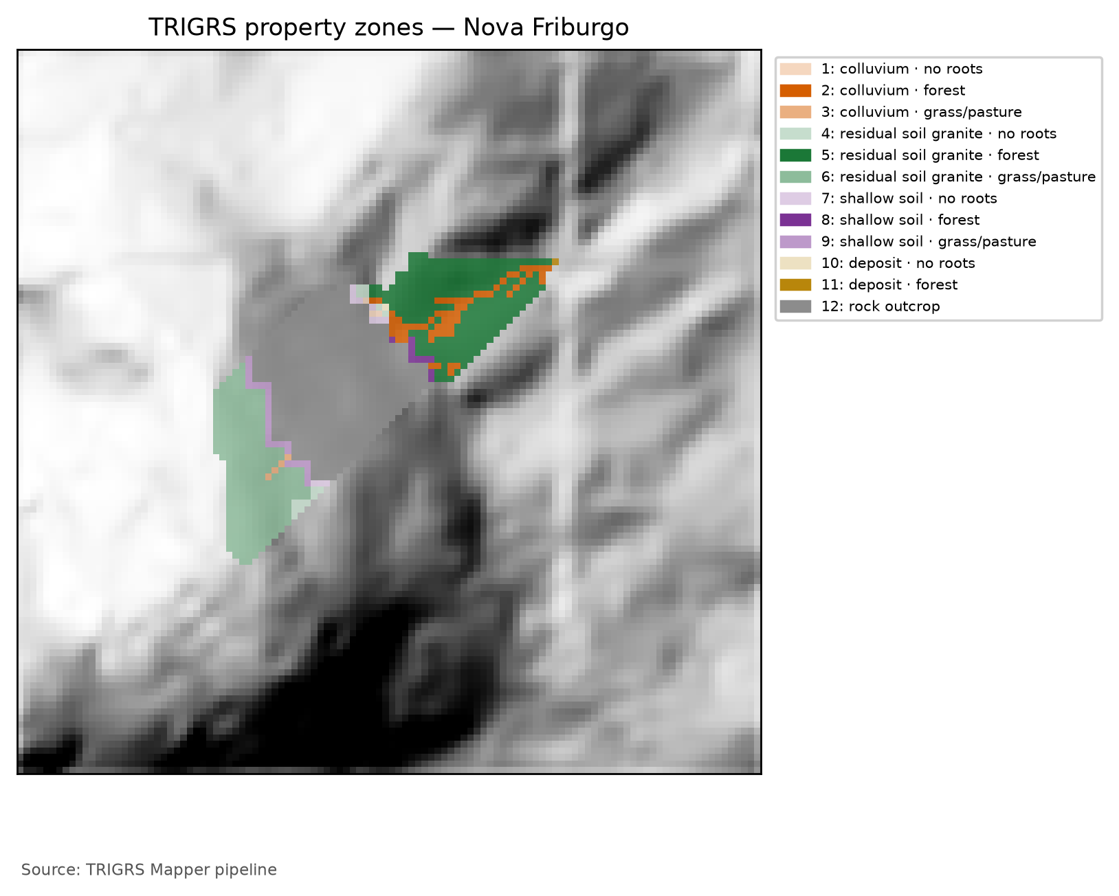
The run of the 2011 event uses the land cover of that time (GLAD 2010), which only distinguishes trees (G1) from short vegetation (G3): the combinations present change, and the zones are numbered differently (Table 6.31). The calibration window uses the same land cover as the event.
tr_in.txt) with the multipliers in use (full calibration, sample lhs_0019: mc = 0.92, mtanφ = 1.04, mKs = 0.70, rD0 = 39 m, mα = 0.57, mCr = 1.42). c′ = c′0·mc and cr = Cr·mCr (total cohesion c = c′ + cr); tan φ′ = mtanφ·tan φ′0; Ks = Ks0·mKs; D0 = rD0·Ks; α = α0·mα; γs derived from θs and Gs. The rock outcrop is the conventional, uncalibrated zone (α < 0: saturated infiltration). The calibration window (30 m) uses the same event land cover.
| Zone · unit (lithology) · land cover | c′ + cr (kPa) | φ′ (°) | γs (kN/m³) | Ks (m/s) | D0 (m²/s) | θs / θr | α (1/m) | Area (%) |
|---|---|---|---|---|---|---|---|---|
| 1 · colluvium · G1 | 2.77 + 2.84 | 34.9 | 18.02 | 7.02 × 10⁻⁶ | 2.74 × 10⁻⁴ | 0.48 / 0.08 | 2.85 | 5.6 |
| 2 · colluvium · G3 | 2.77 + 0.71 | 34.9 | 18.02 | 7.02 × 10⁻⁶ | 2.74 × 10⁻⁴ | 0.48 / 0.08 | 2.85 | 0.6 |
| 3 · mature residual soil (granite) · G1 | 4.61 + 2.84 | 36.0 | 17.81 | 7.02 × 10⁻⁶ | 2.74 × 10⁻⁴ | 0.50 / 0.10 | 3.99 | 23.3 |
| 4 · mature residual soil (granite) · G3 | 4.61 + 0.71 | 36.0 | 17.81 | 7.02 × 10⁻⁶ | 2.74 × 10⁻⁴ | 0.50 / 0.10 | 3.99 | 22.8 |
| 5 · shallow soil over rock · G1 | 1.84 + 2.84 | 38.0 | 18.50 | 1.40 × 10⁻⁵ | 5.49 × 10⁻⁴ | 0.45 / 0.06 | 3.42 | 1.3 |
| 6 · shallow soil over rock · G3 | 1.84 + 0.71 | 38.0 | 18.50 | 1.40 × 10⁻⁵ | 5.49 × 10⁻⁴ | 0.45 / 0.06 | 3.42 | 3.0 |
| 7 · talus/alluvium deposit · G1 | 0.92 + 2.84 | 37.0 | 19.60 | 3.51 × 10⁻⁵ | 1.37 × 10⁻³ | 0.38 / 0.05 | 4.56 | 0.2 |
| 8 · rock outcrop | 100.00 + 0.00 | 45.0 | 26.00 | 1.00 × 10⁻⁹ | 1.00 × 10⁻⁷ | 0.05 / 0.01 | < 0 (sat.) | 43.1 |
6.8.3 Soil thickness: the zmax model
In TRIGRS, zmax is the impermeable base of the profile: the lower limit of infiltration and of the failure surfaces tested. In the Rio de Janeiro Highlands, the best physical match is the discontinuity between the colluvium or the lateritic soil and the saprolite (or the rock), at a depth of 1–2.5 m: this is where the 0.5 to 2.0 m deep landslides of 2011 formed (Marques et al., 2017), as did the failure of the lateritic layer studied by Machado (2016). It is not the depth to sound bedrock — the 25.7–29.1 m of BDTICM (Figure 6.12) measure the whole regolith, including the saprolite that is not mobilized in a shallow landslide.
Without thickness measurements in the watershed, zmax comes from an exponential function of slope δ (in degrees), anchored on the regional evidence (2.0 m at 30° and 1.0 m at 50°):
\[ z_{max} = \min\left\{5;\ \max\left[0.3;\ 5.66\,m_z\,e^{-k_z\,\delta}\right]\right\}\ \text{m}, \]
with \(m_z\) = 1 and \(k_z\) = 0.0347 degree⁻¹ a priori and caps of 0.5 m on the shallow soil and 0.1 m on the outcrop. The BDTICM depth to bedrock (25.7–29.1 m) lies far above the 5 m cap: it does not limit zmax and serves, rescaled, only as an alternative spatial pattern in the sensitivity analysis. For δ ≥ 30° the curve differs by less than 0.35 m from that of DeRose (1996), used in TRIGRS applications (Salciarini et al., 2006) (Table 6.32). The two coefficients become calibratable parameters, \(m_z\) ∈ [0.6; 1.4] and \(k_z\) ∈ [0.025; 0.045] degree⁻¹; the calibrated configuration uses \(m_z\) = 0.62 and \(k_z\) = 0.0269 degree⁻¹ (Figure 6.32).
zmax from the adopted exponential model (a priori: \(m_z\) = 1 and \(k_z\) = 0.0347 degree⁻¹) and from the DeRose (1996) curve.
| δ (°) | 10 | 20 | 30 | 40 | 50 | 60 |
|---|---|---|---|---|---|---|
| adopted model, a priori (m) | 4.00 | 2.83 | 2.00 | 1.41 | 1.00 | 0.71 |
| DeRose (1996): 7.72·e^(−0.04·δ) (m) | 5.17 | 3.47 | 2.33 | 1.56 | 1.04 | 0.70 |
WarningThickness from slope alone is the weakest option
Segoni et al. (2012) compared five soil-thickness models in two areas and concluded that the one derived from slope alone was the worst predictor of landslides. That is why the sensitivity analysis (Section 6.9.7) replaces zmax with the DeRose curve, with uniform thicknesses of 1.25 and 2.0 m, with a linear relationship, and with the rescaled spatial pattern of BDTICM. Measurements — boreholes, trenches, differences between DEMs before and after an event — are the cheapest improvement for this model (Section 6.11.3).
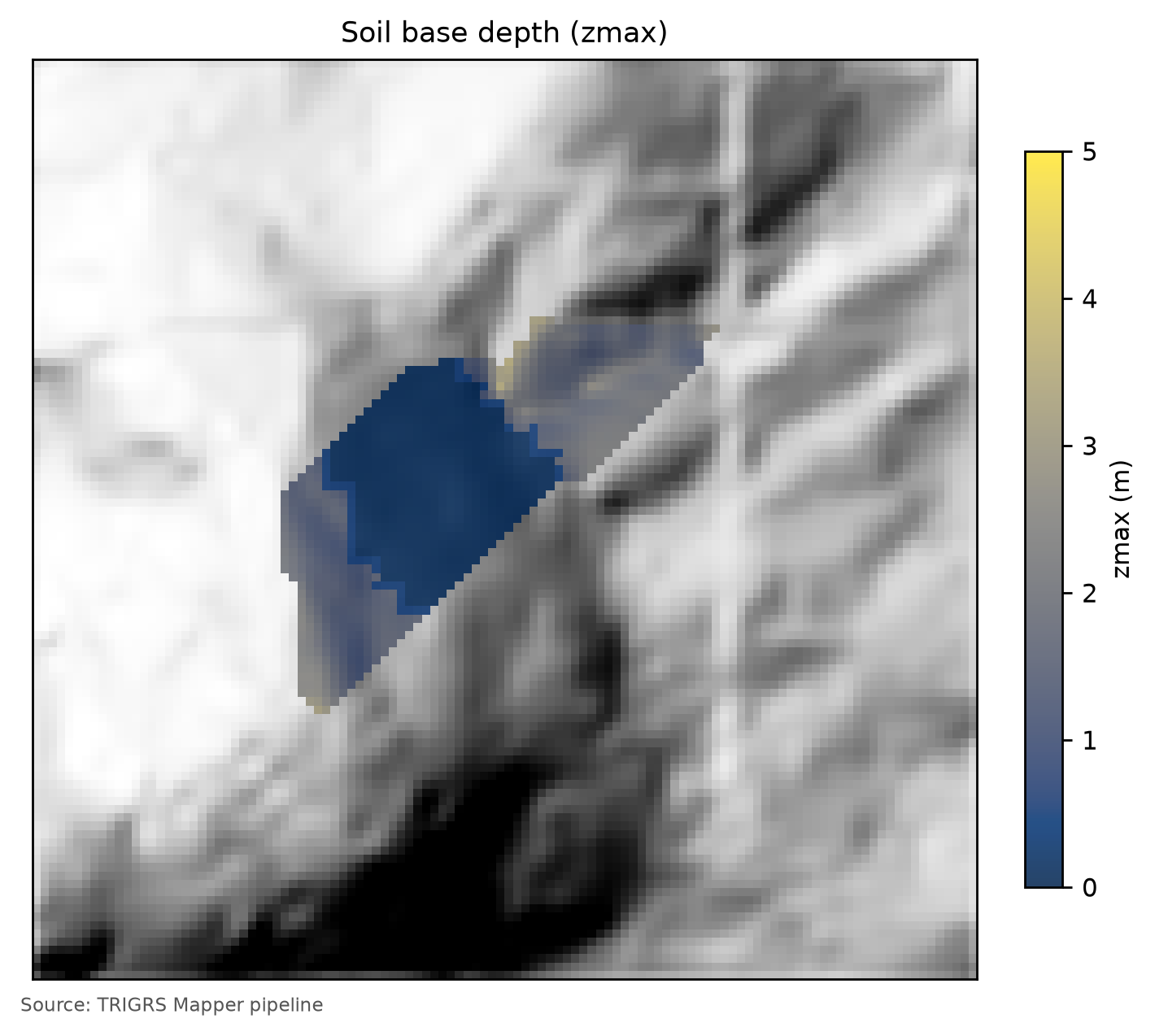
zmax, m) on the 10 m watershed, with the calibrated parameters (\(m_z\) and \(k_z\)). The outcrop (0.1 m cap) and the shallow-soil strip (0.5 m cap) appear in dark blue; on the soil-mantled hillslopes the thickness decreases with slope, and the gentlest reaches hit the 5 m cap.
6.8.4 Initial water table and background infiltration
TRIGRS does not start the run “from nothing”: before the first rain, the profile is in a steady state defined by the initial depth of the water table \(d\) (depthwt) and by the background infiltration \(I_{ZLT}\) (rizero) — the recharge rate that sustained this state over the preceding days and months. Below the water table, the initial pressure head corresponds to slope-parallel flow (Iverson, 2000; Baum et al., 2008):
\[ \psi_0(Z) = (Z - d)\left(\cos^2\delta - \frac{I_{ZLT}}{K_s}\right), \]
and, above it, the unsaturated model starts from a suction profile in equilibrium with \(I_{ZLT}\). The rainfall adds the transient part to this state.
The initial condition also has a factor of safety. With \(\psi_0(Z)\) in place of \(\psi(Z,t)\), the same infinite-slope equation (Chapter 1) gives the FS of the steady state, \(FS_0 = FS(Z, t = 0)\), which tells whether the slope stands before any rainfall. The pipeline computes the FS0 of each cell in closed form, reproducing the TRIGRS routines for t = 0 without running the program (trigrs_mapper.trigrs.fs_inicial, validated against the executable; decision D21). Hence two categories of unstable cell:
- unstable at the initial condition: \(FS_0 < 1\) — the model has it failing without any rain;
- triggered by the rainfall: \(FS_0 \ge 1\) and minimum FS < 1 during the run — the failure that the rainfall causes.
This split guides the choice of parameters (Section 6.9.4), the volumes (Section 6.10.4), and the thresholds (Section 6.10.7). It does not depend on the numerical accuracy of the series of the unsaturated model (Section 6.8.6): the state at t = 0 does not use these series.
Initial water table. There are no water-table measurements on the hillslopes of the Rio de Janeiro Highlands before 2011. By project decision (D6), the initial water table is handled through scenarios \(d\) = 1, 2, …, 10 m, capped at the soil base: depthwt = min(\(d\), zmax). Since zmax ≤ 5 m, any \(d\) ≥ 5 m is equivalent to the water table at the base — the a priori case, the practice of Vieira et al. (2010) and of Listo et al. (2018) —, and, on slopes steeper than ~30°, where the a priori zmax is less than 2 m, even \(d\) = 2 m is already the base (Figure 6.33). In the calibration, the water table enters as a fraction of the thickness, depthwt = \(f_{NA}\)·zmax, with \(f_{NA}\) ∈ {0.5; 0.75; 1.0}: with the water table at the base and the central α, the profile above the capillary fringe is dry, the 2011 rainfall does not saturate it, and the a priori model is too stable. The calibrated configuration uses \(f_{NA}\) = 0.50.
Background infiltration. rizero comes from the antecedent rainfall (Section 6.5.7): in Nova Friburgo, the net rate over the 30 days before the event exceeded the 5 × 10⁻⁸ m/s cap of the recommended range (1 × 10⁻⁹ to 5 × 10⁻⁸ m/s), and the suggested value is the cap itself — the value of the a priori run, 5.00 × 10⁻⁸ m/s. In the calibration, rizero is sampled within this range, on a logarithmic scale; the calibrated value is 1.47 × 10⁻⁹ m/s. In each cell, rizero ≤ 0.5·Ks, because TRIGRS requires rizero < Ks.
NoteThe initial water table is an effective parameter
The calibrated \(f_{NA}\) is not a measured water table: it is an effective parameter (decision D21). It represents the moisture left by the rains of the weeks before the event (Table 6.21), but it also compensates for simplifications of the model, which is one-dimensional and has no lateral flow. Small fractions, such as the water table at mid-thickness — that of the calibrated configuration, \(f_{NA}\) = 0.50 —, can leave steep slopes with \(FS_0 < 1\), unstable before the rain begins; the calibration only accepts parameter sets in which these cells stay below the limits of the filters (box “Unstable before the rain”, in Section 6.9.4). The design runs inherit the calibrated initial condition — \(f_{NA}\) and rizero — and keep it the same in the present and in the future: the volumes in this chapter hold for a storm onset as wet as that of January 2011.
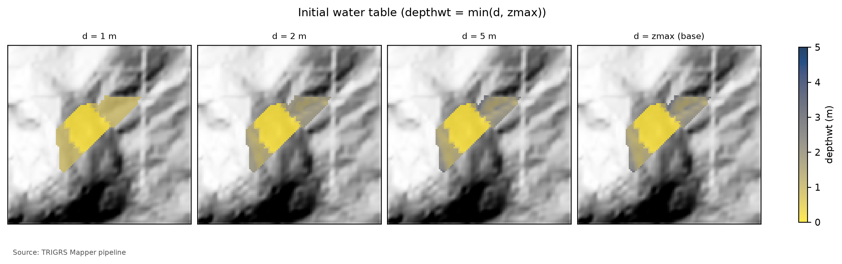
depthwt = min(\(d\), zmax) on the 10 m watershed for \(d\) = 1, 2, and 5 m and for the water table at the soil base (\(d\) = zmax, the a priori value). Light colors indicate a shallow water table. With \(d\) = 5 m almost the whole watershed already has the water table at the base; the calibrated configuration uses depthwt = \(f_{NA}\)·zmax.
6.8.5 Gardner’s unsaturated model
The 2011 landslides in Nova Friburgo were attributed to the loss of suction as the wetting front advanced and to a perched water table over the less permeable contact (Oliveira, 2013; Machado, 2016) — processes that depend on water storage in the unsaturated zone. For this reason, the main configuration is the TRIGRS unsaturated, finite-depth model (Baum et al., 2010), activated in the zones with α > 0. Above the water table, conductivity and water content follow Gardner’s (1958) exponential model, which has an analytical solution for transient vertical infiltration (Srivastava and Yeh, 1991):
\[ K(\psi) = K_s\,e^{\alpha\psi}, \qquad \theta(\psi) = \theta_r + (\theta_s - \theta_r)\,e^{\alpha\psi}, \qquad \psi \le 0, \]
where ψ is the pressure head (negative = suction). The parameter α controls how quickly the soil loses water as suction increases, and \(1/\alpha\) gives the order of magnitude of the capillary fringe: 0.2 m for α = 5 m⁻¹ and 1 m for α = 1 m⁻¹. To compare with van Genuchten retention curves, \(\alpha_G \approx 1.3\,\alpha_{vG}\,n\) (Ghezzehei et al., 2007). In Nova Friburgo, the curves measured on structured mature soils give 12–16 m⁻¹ and the Guelph permeameter 18–23 m⁻¹ (Oliveira, 2013), whereas the Rosetta pedotransfer function (Zhang and Schaap, 2017) predicts 1.3–3 m⁻¹ for the same textures. The a priori values (5 to 8 m⁻¹, Table 6.29) lie between the two and are adjusted by the multiplier \(m_\alpha\) ∈ [0.5; 2], calibrated at 0.57.
In the zones with α ≤ 0 — here, only the outcrop —, TRIGRS uses the saturated model (Iverson, 2000; Baum et al., 2008), without storage in the unsaturated zone. The fully saturated mode, faster and more conservative, enters the sensitivity analysis.
6.8.6 Discretization, run control, and the tr_in.txt file
The control choices follow the project’s parameter report and the convergence tests of the pipeline (docs/METODO-PIPELINE.md, §5 and §10):
- Depth. The profile of each cell is divided into
nzsincrements, Δz = (zmax−zmin)/nzs, which define the resolution of \(Z_{cr}\):nzs= 20 in the calibration, sensitivity, and threshold runs, and 30 in the final watershed runs, for the event and the design storms (D20), which gives Δz ≤ 0.1 m forzmax≤ 3 m.zmin= 0.1 m discards irrelevant, very shallow failures. - Time. In the unsaturated model the time step is uniform, Δt = t/(nper·tx). We use
tx= 1 in the calibration and design runs (Table 6.33); when there are few rainfall periods (the thresholds, with uniform rainfall in a single period) or frequent FS frames (the event on the watershed), the pipeline raisestxso that the time step stays on the order of the interval between outputs. The output times are rounded to multiples of Δt, instead of letting TRIGRS change them silently; convergence was checked withtx= 3 and 5. - Series.
mmax= 100 terms, andnmax= 100 in the 151 calibration runs and 300 in the later steps — event, design, sensitivity, and thresholds (D21). With 30 terms, some cells of a test in Petrópolis did not converge in the unsaturated zone; with 100, none did. In the Nova Friburgo window, however, a sample with low Ks and high α still left about a third of the cells without convergence with 100 terms — all of them stable, with no change of FS class —, and with 300 none, at +1.5% CPU (D21 test). Sincenmaxenters the run signature, the calibration runs kept 100, and the fraction of non-converging cells of each sample became a numerical-validity filter of the selection (Section 6.9.4). The manifests record the non-converging cells of each run. - Minimum slope.
Min_Slope_Angle= 10° in the runs of the calibration phase (window, sensitivity, and thresholds): even with saturated soil and slope-parallel flow, c′ ≥ 0 and φ′ ≥ 21° require δ ≳ 10° for FS < 1, and the flatter cells would only cost time. In the final watershed runs, 0°. - Flow direction.
flowdir=gener, the general case of TRIGRS; thehydrooption, without drainage through the base, enters the sensitivity analysis. - Post-rain window. The design and threshold runs simulate 24 h without rain after the hyetograph: in the central colluvium, the wetting front takes \(Z(\theta_s-\theta_r)/K_s \approx 2 \times 0.40/10^{-5}\) s ≈ 22 h to reach 2 m, and instability can appear after the rain ends. The design FS is the minimum over time.
- Outputs. Minimum FS of the profile, \(Z_{cr}\), and pressure head at \(Z_{cr}\) at each output time. The grid of the computed water table is not requested, because it differs between serial and parallel TRIGRS (D11).
- Runoff and parallelism. Before each run, TopoIndex computes the computation order and the weights of the D8 routing of surface runoff (Chapter 5): rain in excess of Ks runs off to the cells downslope. The event run on the 10 m watershed uses TRIGRS-P (Alvioli and Baum, 2016), the parallel (MPI) version, which exactly reproduced the serial one on a grid of 160 thousand cells (D13).
Table 6.33 compares the control parameters of the tr_in.txt files actually run — the design run for T = 100 years in the present climate and the best calibration run —, and the collapsible box that follows shows the whole design file, annotated line by line. Compare with the tr_in.txt of the tutorial example (Chapter 4): the structure is the same; what changes is the number of zones, the rainfall (24 one-hour blocks followed by the rain-free window), and the fact that zmax, depth, and rizero come from grids (value −1 in the line marked 4).
tr_in.txt files: design run in the watershed (data/cases/nova_friburgo/runs/projeto/tr100_presente_atual_obs/tr_in.txt) and best calibration run in the window (data/cases/nova_friburgo/runs/calibracao/lhs/lhs_0019/tr_in.txt).
| Parameter | Design run — 10 m watershed (100-yr, present) | Calibration — 30 m window (best sample) | Meaning |
|---|---|---|---|
| Infiltration model | unsaturated, finite depth (unsfin) |
unsaturated, finite depth (unsfin) |
α > 0 in the soil zones; α ≤ 0 (outcrop) → saturated infiltration |
nzs |
30 | 20 | depth increments (Δz ≈ zmax/nzs) |
tx |
1 | 1 | time-step subdivision |
nmax |
300 | 100 | maximum number of series terms (convergence) |
mmax |
100 | 100 | maximum number of series terms (convergence) |
zmin (m) |
0.10 | 0.10 | minimum computation depth |
Min_Slope_Angle (°) |
0 | 10 | flatter cells are not analyzed |
flowdir |
gener |
gener |
infiltration flow direction |
nper (rainfall periods) |
24 | 26 | rainfall blocks of the run |
t (h) |
48.0 | 96.0 | simulated duration (rain + rain-free window) |
| Δt = t/(kper·tx) (h) | 1.92 | 3.69 | time step of the unsaturated model |
| Output times | 24 | 4 | grids written during the run |
| Zones (saturated) | 12 (1) | 15 (1) | property zones (with α ≤ 0) |
TipThe actual
tr_in.txt of the design run (100-yr, present), annotated line by line
File data/cases/nova_friburgo/runs/projeto/tr100_presente_atual_obs/tr_in.txt, written by trigrs_mapper.trigrs and read by TRIGRS 2.1. The text lines are labels that the program reads and ignores; each number below the block annotates the marked line of values. The zones are those of the design parameterization (land cover MapBiomas 2025; 12 zones), numbered as in the design zone table; the event run and the calibration use the event land cover (GLAD GLCLUC 2010; 8 zones in the watershed) and a different numbering (event zone table).
tr_in.txt
Name of project (up to 255 characters)
1TRIGRS Mapper nova_friburgo bacia 10 m
tx, nmax, mmax, zones
21, 300, 100, 12
nzs,  zmin,  uww,    nper    t
330, 0.1, 9810.0, 24, 172800.0
zmax,   depth,   rizero,  Min_Slope_Angle (degrees), Max_Slope_Angle (degrees)
4-1.0, -1.0, -1.0, 0.0, 90.0
zone, 1
cohesion,phi,  uws,   diffus,   K-sat, Theta-sat,Theta-res,Alpha
52765.7664654352748, 34.945633774205305, 18022.932, 0.0002744201025695286, 7.015609100955407e-06, 0.48, 0.08, 2.8497359566952434
zone, 2
cohesion,phi,  uws,   diffus,   K-sat, Theta-sat,Theta-res,Alpha
65602.637438498691, 34.945633774205305, 18022.932, 0.0002744201025695286, 7.015609100955407e-06, 0.48, 0.08, 2.8497359566952434
zone, 3
cohesion,phi,  uws,   diffus,   K-sat, Theta-sat,Theta-res,Alpha
73474.984208701129, 34.945633774205305, 18022.932, 0.0002744201025695286, 7.015609100955407e-06, 0.48, 0.08, 2.8497359566952434
zone, 4
cohesion,phi,  uws,   diffus,   K-sat, Theta-sat,Theta-res,Alpha
84609.610775725458, 35.95783354114205, 17805.149999999998, 0.0002744201025695286, 7.015609100955407e-06, 0.5, 0.1, 3.989630339373341
zone, 5
cohesion,phi,  uws,   diffus,   K-sat, Theta-sat,Theta-res,Alpha
97446.481748788874, 35.95783354114205, 17805.149999999998, 0.0002744201025695286, 7.015609100955407e-06, 0.5, 0.1, 3.989630339373341
zone, 6
cohesion,phi,  uws,   diffus,   K-sat, Theta-sat,Theta-res,Alpha
105318.828518991311, 35.95783354114205, 17805.149999999998, 0.0002744201025695286, 7.015609100955407e-06, 0.5, 0.1, 3.989630339373341
zone, 7
cohesion,phi,  uws,   diffus,   K-sat, Theta-sat,Theta-res,Alpha
111843.844310290183, 37.978659128023935, 18496.755, 0.0005488402051390572, 1.4031218201910814e-05, 0.45, 0.06, 3.4196831480342924
zone, 8
cohesion,phi,  uws,   diffus,   K-sat, Theta-sat,Theta-res,Alpha
124680.715283353599, 37.978659128023935, 18496.755, 0.0005488402051390572, 1.4031218201910814e-05, 0.45, 0.06, 3.4196831480342924
zone, 9
cohesion,phi,  uws,   diffus,   K-sat, Theta-sat,Theta-res,Alpha
132553.0620535560374, 37.978659128023935, 18496.755, 0.0005488402051390572, 1.4031218201910814e-05, 0.45, 0.06, 3.4196831480342924
zone, 10
cohesion,phi,  uws,   diffus,   K-sat, Theta-sat,Theta-res,Alpha
14921.9221551450916, 36.96884583477373, 19602.341999999997, 0.001372100512847643, 3.5078045504777035e-05, 0.38, 0.05, 4.55957753071239
zone, 11
cohesion,phi,  uws,   diffus,   K-sat, Theta-sat,Theta-res,Alpha
153758.793128208508, 36.96884583477373, 19602.341999999997, 0.001372100512847643, 3.5078045504777035e-05, 0.38, 0.05, 4.55957753071239
zone, 12
cohesion,phi,  uws,   diffus,   K-sat, Theta-sat,Theta-res,Alpha
16100000.0, 45.0, 26000.0, 1e-07, 1e-09, 0.05, 0.01, -1.0
cri(1), cri(2), ..., cri(nper)
175.540555555555555e-07, 5.95e-07, 6.436666666666667e-07, 7.02611111111111e-07, 7.757222222222222e-07, 8.193611111111111e-07, 8.691388888888889e-07, 1.126111111111111e-06, 1.7030277777777777e-06, 2.3883333333333335e-06, 3.6225e-06, 2.2669277777777775e-05, 5.25575e-06, 2.85175e-06, 2.074e-06, 1.5354444444444443e-06, 1.0328611111111112e-06, 8.392222222222221e-07, 7.800277777777777e-07, 7.370833333333334e-07, 6.716666666666667e-07, 6.182222222222223e-07, 5.736944444444445e-07, 5.359166666666666e-07
capt(1), capt(2), ..., capt(n), capt(n+1)
180.0, 3600.0, 7200.0, 10800.0, 14400.0, 18000.0, 21600.0, 25200.0, 28800.0, 32400.0, 36000.0, 39600.0, 43200.0, 46800.0, 50400.0, 54000.0, 57600.0, 61200.0, 64800.0, 68400.0, 72000.0, 75600.0, 79200.0, 82800.0, 86400.0
File name of slope angle grid (slofil)
19data/slope.asc
File name of digital elevation grid (elevfil)
20data/dem.asc
File name of property zone grid (zonfil)
21data/zones.asc
File name of depth grid (zfil)
22data/zmax.asc
File name of initial depth of water table grid   (depfil)
23data/depthwt.asc
File name of initial infiltration rate grid   (rizerofil)
24data/rizero.asc
List of file name(s) of rainfall intensity for each period, (rifil())
25none
none
none
none
none
none
none
none
none
none
none
none
none
none
none
none
none
none
none
none
none
none
none
none
File name of grid of D8 runoff receptor cell numbers (nxtfil)
26data/TIdscelGrid_prj.txt
File name of list of cells defining runoff computation order (ndxfil)
27data/TIcelindxList_prj.txt
File name of list of all runoff receptor cells  (dscfil)
28data/TIdscelList_prj.txt
File name of list of runoff weighting factors  (wffil)
29data/TIwfactorList_prj.txt
Folder where output grid files will be stored  (folder)
30Resultados/
Identification code to be added to names of output files (suffix)
31prj
Save grid files of runoff? Enter T (.true.) or F (.false.)
32F
Save grid of minimum factor of safety? Enter T (.true.) or F (.false.)
33T
Save grid of depth of minimum factor of safety? Enter T (.true.) or F (.false.)
34T
Save grid of pressure head at depth of minimum factor of safety? Enter T (.true.) or F (.false.)
35T
Save grid of computed water table depth or elevation? Enter T (.true.) or F (.false.) followed by 'depth,' or 'eleva'
36F, depth
Save grid files of actual infiltration rate? Enter T (.true.) or F (.false.)
37F
Save grid files of unsaturated zone basal flux? Enter T (.true.) or F (.false.)
38F
Save listing of pressure head and factor of safety ("flag")? (-9 sparse xmdv , -8 down-sampled xmdv, -7 full xmdv, -6 sparse ijz, -5 down-sampled ijz, -4 full ijz, -3 Z-P-Fs-saturation list -2 detailed Z-P-Fs, -1 Z-P-Fs list, 0 none). Enter flag value followed by down-sampling interval (integer).
390, 1
Number of times to save output grids and (or) ijz/xmdv files
4024
Times of output grids and (or) ijz / xmdv files
416912.0, 13824.0, 20736.0, 27648.0, 34560.0, 41472.0, 48384.0, 55296.0, 62208.0, 69120.0, 76032.0, 82944.0, 96768.0, 103680.0, 110592.0, 117504.0, 124416.0, 131328.0, 138240.0, 145152.0, 152064.0, 158976.0, 165888.0, 172800.0
Skip other timesteps? Enter T (.true.) or F (.false.)
42F
Use analytic solution for fillable porosity?  Enter T (.true.) or F (.false.)
43T
Estimate positive pressure head in rising water table zone (i.e. in lower part of unsat zone)?  Enter T (.true.) or F (.false.)
44T
Use psi0=-1/alpha? Enter T (.true.) or F (.false.) (False selects the default value, psi0=0)
45F
Log mass balance results?   Enter T (.true.) or F (.false.)
46F
Flow direction (Enter "gener", "slope", or "hydro")
47gener
Add steady background flux to transient infiltration rate to prevent drying beyond the initial conditions during periods of zero infiltration?
48T
Specify file extension for output grids. Enter T (.true.) for ".asc" or F for ".txt"
49T
Ignore negative pressure head in computing factor of safety (saturated infiltration only)?   Enter T (.true.) or F (.false.)
50T
Ignore height of capillary fringe in computing pressure head for unsaturated infiltration option?   Enter T (.true.) or F (.false.)
51T
Parameters for deep pressure-head estimate in SCOOPS ijz output: Depth below ground surface (positive, use negative value to cancel this option), pressure option (enter 'zero' , 'flow' , 'hydr' , or 'relh')
52-50.0, flow- 1
- Run title (free text, up to 255 characters).
- 2
-
tx= 1: time-step subdivision (unsaturated model: Δt = t/(kper·tx), kper = number of periods; TRIGRS increasestxwhen needed to separate the output times);nmax= 300 andmmax= 100: maximum number of terms in the series of the infiltration solutions;zones= 12 property zones. - 3
-
nzs= 30 depth increments (Δz ≈ zmax/30);zmin= 0.1 m (minimum computation depth);uww= 9,810 N/m³ (unit weight of water);nper= 24 rainfall periods;t= 172,800 s = 48.0 h simulated (24.0 h of rain + 24.0 h without rain). - 4
-
Negative values:
zmax,depthandrizeroare read cell by cell from the gridszmax.asc,depthwt.ascandrizero.asc; slopes analyzed from 0° to 90° (Min_Slope_Angle,Max_Slope_Angle). - 5
- Zone 1 (colluvium, G0 no roots): c = 2,766 Pa (c′ + root cohesion), φ′ = 34.9°, γs = 18,023 N/m³, D0 = 2.74 × 10⁻⁴ m²/s, Ks = 7.02 × 10⁻⁶ m/s, θs = 0.48, θr = 0.08, α = 2.85 1/m.
- 6
- Zone 2 (colluvium, G1 forest): c = 5,603 Pa (c′ + root cohesion), φ′ = 34.9°, γs = 18,023 N/m³, D0 = 2.74 × 10⁻⁴ m²/s, Ks = 7.02 × 10⁻⁶ m/s, θs = 0.48, θr = 0.08, α = 2.85 1/m.
- 7
- Zone 3 (colluvium, G3 grassland/pasture): c = 3,475 Pa (c′ + root cohesion), φ′ = 34.9°, γs = 18,023 N/m³, D0 = 2.74 × 10⁻⁴ m²/s, Ks = 7.02 × 10⁻⁶ m/s, θs = 0.48, θr = 0.08, α = 2.85 1/m.
- 8
- Zone 4 (mature residual soil, granite, G0 no roots): c = 4,610 Pa (c′ + root cohesion), φ′ = 36.0°, γs = 17,805 N/m³, D0 = 2.74 × 10⁻⁴ m²/s, Ks = 7.02 × 10⁻⁶ m/s, θs = 0.50, θr = 0.10, α = 3.99 1/m.
- 9
- Zone 5 (mature residual soil, granite, G1 forest): c = 7,446 Pa (c′ + root cohesion), φ′ = 36.0°, γs = 17,805 N/m³, D0 = 2.74 × 10⁻⁴ m²/s, Ks = 7.02 × 10⁻⁶ m/s, θs = 0.50, θr = 0.10, α = 3.99 1/m.
- 10
- Zone 6 (mature residual soil, granite, G3 grassland/pasture): c = 5,319 Pa (c′ + root cohesion), φ′ = 36.0°, γs = 17,805 N/m³, D0 = 2.74 × 10⁻⁴ m²/s, Ks = 7.02 × 10⁻⁶ m/s, θs = 0.50, θr = 0.10, α = 3.99 1/m.
- 11
- Zone 7 (shallow soil over rock, G0 no roots): c = 1,844 Pa (c′ + root cohesion), φ′ = 38.0°, γs = 18,497 N/m³, D0 = 5.49 × 10⁻⁴ m²/s, Ks = 1.40 × 10⁻⁵ m/s, θs = 0.45, θr = 0.06, α = 3.42 1/m.
- 12
- Zone 8 (shallow soil over rock, G1 forest): c = 4,681 Pa (c′ + root cohesion), φ′ = 38.0°, γs = 18,497 N/m³, D0 = 5.49 × 10⁻⁴ m²/s, Ks = 1.40 × 10⁻⁵ m/s, θs = 0.45, θr = 0.06, α = 3.42 1/m.
- 13
- Zone 9 (shallow soil over rock, G3 grassland/pasture): c = 2,553 Pa (c′ + root cohesion), φ′ = 38.0°, γs = 18,497 N/m³, D0 = 5.49 × 10⁻⁴ m²/s, Ks = 1.40 × 10⁻⁵ m/s, θs = 0.45, θr = 0.06, α = 3.42 1/m.
- 14
- Zone 10 (talus/alluvium deposit, G0 no roots): c = 922 Pa (c′ + root cohesion), φ′ = 37.0°, γs = 19,602 N/m³, D0 = 1.37 × 10⁻³ m²/s, Ks = 3.51 × 10⁻⁵ m/s, θs = 0.38, θr = 0.05, α = 4.56 1/m.
- 15
- Zone 11 (talus/alluvium deposit, G1 forest): c = 3,759 Pa (c′ + root cohesion), φ′ = 37.0°, γs = 19,602 N/m³, D0 = 1.37 × 10⁻³ m²/s, Ks = 3.51 × 10⁻⁵ m/s, θs = 0.38, θr = 0.05, α = 4.56 1/m.
- 16
- Zone 12 (rock outcrop): c = 100,000 Pa (conventional, uncalibrated zone), φ′ = 45.0°, γs = 26,000 N/m³, D0 = 1.00 × 10⁻⁷ m²/s, Ks = 1.00 × 10⁻⁹ m/s, θs = 0.05, θr = 0.01, α = −1.00 1/m (α ≤ 0: saturated infiltration in this zone).
- 17
-
Intensity
criof each of the 24 periods (m/s; × 3.6 × 10⁶ = mm/h): peak of 81.6 mm/h, total of 194.3 mm. - 18
-
Start of each period and end of rain (
capt, s): 24.0 h of rain in 1.0-h blocks. - 19
- Slope grid (degrees).
- 20
- Conditioned DEM (the one used by TopoIndex).
- 21
- Property-zone grid (1…N).
- 22
-
Depth of the impermeable base
zmax(m), per cell. - 23
- Initial water-table depth (m), per cell.
- 24
-
Initial (steady) infiltration
rizero(m/s), per cell. - 25
-
One line per period (24):
none= no rainfall grid — the uniform intensitycriof the period is used. - 26
- TopoIndex: D8 receptor cell of each cell (runoff routing).
- 27
- TopoIndex: runoff computation order.
- 28
- TopoIndex: list of receptor cells.
- 29
- TopoIndex: runoff weighting factors.
- 30
- Output-grid folder (it must exist before the run).
- 31
- Suffix of the output-grid names.
- 32
- Grades de escoamento: no.
- 33
- Grid of the minimum FS in the profile at each output time: yes.
- 34
- Depth of the minimum FS, Z_cr (basis of V_TRIGRS): yes.
- 35
- Pressure head at the depth of the minimum FS: yes.
- 36
- Computed water table: no (this grid differs in TRIGRS-P; D11).
- 37
- Actual infiltration: no.
- 38
- Basal flux of the unsaturated zone: no.
- 39
-
flag= 0: no pressure-head/FS listings by depth. - 40
- 24 output times.
- 41
- Output times (s): from 1.9 h to 48.0 h — the pipeline rounds them to multiples of the time step (METODO-PIPELINE §5).
- 42
- Skip the time steps between outputs: no.
- 43
- Analytic solution for the fillable porosity (rising water table): yes.
- 44
- Positive pressure head in the lower unsaturated zone as the water table rises: yes.
- 45
- ψ0 = −1/α: no (F = default, ψ0 = 0).
- 46
- Mass-balance log: no (costs ~12 % of the run time; METODO-PIPELINE §10).
- 47
-
Infiltration flow direction:
gener(gener= general case;slopeandhydroare the alternatives;hydrois tested in the sensitivity analysis). - 48
- Add the steady background flux to the transient infiltration (prevents drying beyond the initial condition without rain): yes.
- 49
-
.ascextension for the output grids: yes. - 50
- Ignore negative pressure head in the FS (saturated infiltration only): yes.
- 51
- Ignore the capillary-fringe height in the pressure head (unsaturated infiltration): yes.
- 52
- Scoops3D option (deep pressure head) disabled: negative depth.
6.8.7 Runs performed
Table 6.34 summarizes the run plan of the case. The calibration and the sensitivity analysis use the 30 m window; everything that becomes a volume uses the 10 m watershed.
| Step | Domain | Rainfall | Configuration | Runs (full run) | Use |
|---|---|---|---|---|---|
| calibration | window, 30 m | 2011 event: 2 antecedent days + 48 h in 2-h blocks | a priori + Latin hypercube samples | 1 + 150 | choose the multipliers (Section 6.9.4) |
| cross-validation | Teresópolis window, 30 m | 2011 event in Teresópolis | calibrated in Nova Friburgo and a priori | 2 | test the transfer (Section 6.9.6) |
| event | 30 m window and 10 m watershed | 2011 event (on the watershed, FS frames every 2 h) | calibrated | 2 | hits and misses; event volume (Section 6.10.4) |
| sensitivity | 30 m window; watershed at 30 and 10 m; 10 m window | event and variants | calibrated, one factor at a time | ≈ 35 | tornado (Section 6.9.7) |
| design | 10 m watershed | 24-h hyetograph + 24 h without rain | calibrated; MapBiomas 2025 | 8 T × 11 scenarios = 88 | volume × T × climate (Section 6.10.5) |
| thresholds | 10 m watershed | uniform rainfall: 7 durations × 12 accumulations | calibrated; 4 initial water-table conditions | 336 | thresholds of the Forecast tab (Section 6.10.7) |
| initial condition (FS0) | 10 m watershed, in each step | none (t = 0) | that of each run | none: computed in Python | separate the triggered cells from those already unstable at t = 0 (D21) |
In the final run — full mode —, the calibration used 151 runs, the sensitivity analysis 30 variations, and the design step 88 runs (return periods of 2, 5, 10, 25, 50, 100, 200, 500 years; scenarios: present; SSP1-2.6 2071–2100 P50; SSP2-4.5 2041–2070 P50; SSP2-4.5 2071–2100 P50; SSP2-4.5 2071–2100 P10; SSP2-4.5 2071–2100 P90; SSP3-7.0 2071–2100 P50; SSP5-8.5 2041–2070 P50; SSP5-8.5 2071–2100 P50; SSP5-8.5 2071–2100 P10; SSP5-8.5 2071–2100 P90).
6.9 Calibration against the event scars
To calibrate is to choose, among plausible parameter combinations, the one that best reproduces where the slopes failed on January 11–12, 2011 — and when: the failures must be triggered by the rainfall of the event, not already present at the initial condition of the model. We do not adjust each number of the zones of tr_in.txt: we adjust the 10 global multipliers of Section 6.8.2, scoring each combination against the source areas of the scars in the 30 m window. This section shows the rainfall used, the inventory, the metrics, the search, the hit maps, the validation in another area, and the sensitivity analysis — and what all of this teaches.
6.9.1 The event rainfall in TRIGRS
The rainfall is the hyetograph reconstructed in Section 6.5.7 (decision D14): the hourly MERGE shape scaled by the median of the observed totals (Table 6.19), with the daily Xavier antecedent rainfall. Three choices make the 151 runs feasible:
- Antecedent rainfall. Only the last 2 antecedent days enter the transient window; the rest of the rainy month enters through
rizero(Section 6.8.4). - Blocks. The 48 h of the event are aggregated into 2-h blocks (D20); 1-h blocks would triple the cost. The aggregation flattens the peak: 33.9 mm/h as the mean of the most intense block, less than the hourly peak of Table 6.20.
- Outputs. The FS is written at the end of the antecedent period (right before the event rainfall), at the peak, at the end of the rain, at the end of the simulation, and at the reported failure times — 01:00 and 04:00 on January 12, 2011 (Oliveira, 2013). Rounded to multiples of Δt, these instants reduce to the four output times of Table 6.33: the peak coincides with one of the failure times, and the calibration simulation ends with the rain. The event FS is the minimum over these outputs; the one at the end of the antecedent period separates what was already unstable before the event (Section 6.9.3).
In all, there are 26 rainfall periods and 225.4 mm, adding the 2 antecedent days and the event (Figure 6.34). The uncertainty in the event rainfall — the distance between the minimum and maximum scenarios of Table 6.20 — enters the sensitivity analysis.
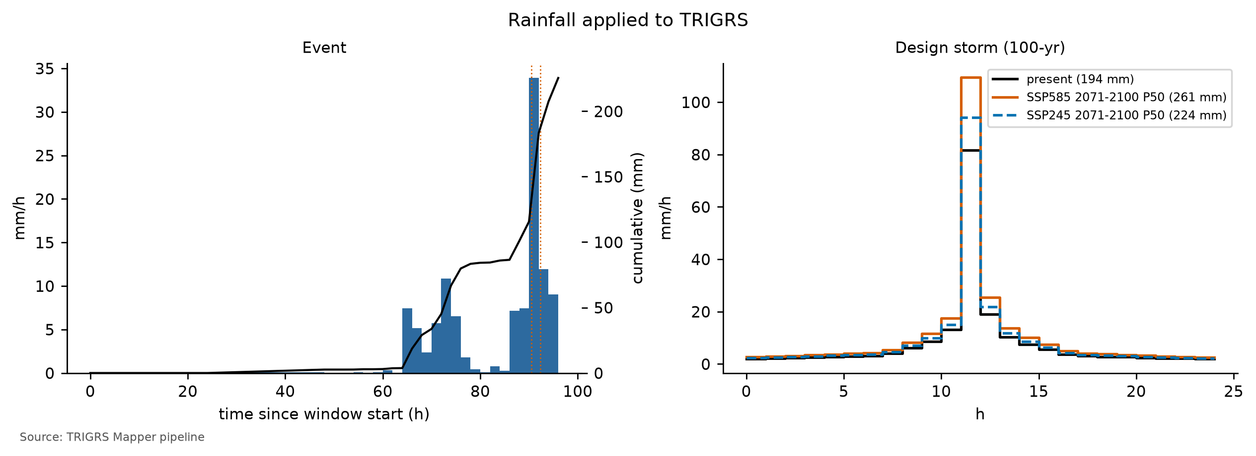
6.9.2 Inventory and source areas
The inventory is that of Marc et al. (2018) and Emberson et al. (2022), not shifted in Nova Friburgo (D17), with 345 scars with a source area in the calibration domain. Each polygon lumps failure, track, and deposit together — the São Lucas Hospital flow is a single 747 m polygon, from the scarp down to the hospital (Section 6.1). Scoring the FS over the whole polygon would count the track and the deposit as misses, although TRIGRS only predicts where the failure starts, not how far the material travels. For this reason the calibration uses an approximate source area: the upper third of each polygon by elevation,
\[ H \ge H_{min} + \tfrac{2}{3}\,(H_{max} - H_{min}), \]
where \(H\) is the DEM elevation inside the polygon. It is a simple, reproducible criterion, confirmed by an independent source: of the scar points of the SGB maps that fall inside the 2011 polygons in Nova Friburgo, 74% lie in the upper third, which covers only 22% of the area of these polygons (project report docs/pesquisa/02_inventarios.md). The window cells are split into:
- positives: 30 m cells with their center in a source area and slope ≥ 10° (at least one per scar) — 528 cells;
- excluded: the rest of each polygon (track and deposit), dilated by one cell — neither positive nor negative;
- negatives: all other window cells — 9,426 cells.
WarningLimitations of the inventory
- The source area is a geometric approximation.
- About 40% of the polygons are smaller than one 30 m cell.
- ANADEM postdates 2011, so the slopes inside the scars are already those of the terrain after the failure.
- An inventory with failure and deposit mapped separately would make it possible to measure the error of these approximations (Section 6.11.3).
6.9.3 Performance metrics
Each run becomes a binary map — unstable if the minimum FS during the event is below 1 — compared cell by cell with the inventory (Table 6.35).
| Scar source area (positive) | Outside the scars (negative) | |
|---|---|---|
| FS < 1 (unstable) | TP — hit | FP — false alarm |
| FS ≥ 1 (stable) | FN — miss | TN — correctly stable |
The four counts yield the metrics used in the calibration:
\[ \begin{aligned} TPR &= \frac{TP}{TP + FN}, & FPR &= \frac{FP}{FP + TN},\\ TNR &= 1 - FPR, & MSR &= \frac{TPR + TNR}{2},\\ TSS &= TPR - FPR = 2\,MSR - 1, & D2PC &= \sqrt{(1 - TPR)^2 + FPR^2},\\ \kappa &= \frac{p_o - p_e}{1 - p_e}, & p_o &= \frac{TP + TN}{N}, \end{aligned} \]
\[ p_e = \frac{(TP + FP)(TP + FN) + (FN + TN)(FP + TN)}{N^2}, \]
where N is the number of evaluated cells.
- TPR (true positive rate) is the fraction of the source areas predicted unstable; FPR, the fraction of the scar-free terrain predicted unstable.
- MSR (modified success rate; Huang and Kao, 2006) is the mean of getting the scars right and getting the stable terrain right: it penalizes the model that “hits” by declaring everything unstable. In its triggered form, defined below, it is the objective function of the calibration (decision D21). TSS is the same criterion on a different scale, and D2PC (Formetta et al., 2016), the distance to the perfect point of the ROC plane — an alternative objective.
- Cohen’s κ (Cohen, 1960) measures agreement beyond chance; with few positive cells, it stays low even for useful models, so it is only informative.
- AUC is the area under the ROC curve (Fawcett, 2006), built by varying the threshold of the −FS score: 0.5 is chance and 1 is perfect ranking (Section 6.9.5).
- Scar detection rate: fraction of the scars with at least one unstable cell in the source area — the scar-level reading, less sensitive to polygon size.
- LRclass (Park et al., 2013): for each FS class, the ratio between the percentage of the scars in the class and the percentage of the area of the class; LR > 1 indicates that the class concentrates scars (Table 6.40, in Section 6.9.5).
TipWhy is the TPR not enough?
A model that declared the whole window unstable would have TPR = 1 — all scars “hit” —, but also FPR = 1, and its MSR would be (1 + 0)/2 = 0.5, the same as chance. The MSR forces the model to be right about where it fails and where it does not. For the same reason, the selection prefers parameter sets with an unstable area of up to 3 times the source area (Section 6.9.4).
The metrics above look at where a cell becomes unstable; others look at when. With the FS of the output at the end of the antecedent period (right before the event rainfall), the pipeline separates the cells that were already unstable before the event from those triggered by it (FS ≥ 1 before and < 1 during the event) and computes the hit rate of the triggered failures only:
\[ TPR_{trig} = \frac{TP_{trig}}{TP + FN}, \qquad MSR_{trig} = \frac{TPR_{trig} + TNR}{2}, \qquad TSS_{trig} = TPR_{trig} - FPR, \]
where \(TP_{trig}\) counts only the source areas that are stable at the end of the antecedent period and unstable during the event. A source area that the model already has unstable before the event counts as a miss: the place is right, but the timing is wrong. Outside the scars, a cell unstable at any time remains a false alarm, so the FPR and the TNR are the same as in the total MSR. Three fractions complete the diagnosis: the evaluated cells and the source cells already unstable before the event, and the share of the event’s unstable cells that were already unstable before it. \(MSR_{trig}\) is the objective function of the calibration, and \(TSS_{trig}\) measures the minimum skill of the chosen configuration (decision D21; Section 6.9.4).
performance metrics of a run (teaching excerpt)
import numpy as np

def metricas(instavel, positiva, negativa, antes=None):
    """Boolean arrays of the window: FS < 1 during the event, source areas, and negative cells (the excluded cells
    are in neither) and, optionally, FS < 1 at the end of the antecedent period (unstable before the event)."""
    vp = np.sum(instavel & positiva);  fn = np.sum(~instavel & positiva)
    fp = np.sum(instavel & negativa);  vn = np.sum(~instavel & negativa)
    tpr, fpr = vp / (vp + fn), fp / (fp + vn)
    n = vp + fn + fp + vn
    po = (vp + vn) / n
    pe = ((vp + fp) * (vp + fn) + (fn + vn) * (fp + vn)) / n**2
    m = {"tpr": tpr, "fpr": fpr, "msr": (tpr + 1 - fpr) / 2, "tss": tpr - fpr,
         "kappa": (po - pe) / (1 - pe), "d2pc": np.hypot(1 - tpr, fpr)}
    if antes is not None:
        vp_d = np.sum(instavel & ~antes & positiva)       # only the scars triggered during the event
        tpr_d = vp_d / (vp + fn)                          # a scar already unstable before counts as a miss
        avaliadas = positiva | negativa
        m |= {"tpr_deflagrado": tpr_d, "msr_deflagrado": (tpr_d + 1 - fpr) / 2,
              "tss_deflagrado": tpr_d - fpr,
              "frac_instavel_pre": np.sum(antes & avaliadas) / n,
              "frac_fonte_instavel_pre": np.sum(antes & positiva) / (vp + fn),
              "frac_instaveis_pre_evento": np.sum(instavel & antes & avaliadas) / (vp + fp)}
    return m
6.9.4 Latin hypercube and choice of the configuration
With 10 parameters, a grid of only three values per parameter would require 3¹⁰ = 59,049 runs. The Latin hypercube (McKay et al., 1979) covers the same space with far fewer: for N samples, the range of each multiplier is divided into N intervals of equal probability, each interval is used exactly once, and the intervals of the different parameters are combined by random permutations. The parameters that vary over orders of magnitude (Ks, \(r_{D0}\), α, and rizero) are sampled on a logarithmic scale, and \(f_{NA}\) only takes the values 0.5, 0.75, and 1.0 (Table 6.36); \(\theta_s\) and \(G_s\) stay at their central values. The full run evaluates 150 samples plus the a priori configuration (D20), with the same seed (20261031) in the three case studies — so the same sample can be compared across watersheds (Section 6.9.6). The results come from 150 samples (full calibration, sample lhs_0019).
calibration.py (excerpt) — Latin hypercube of the multipliers
from trigrs_mapper.calibration import amostras_lhs, faixas_calibracao

faixas = faixas_calibracao()     # m_c, m_tanphi, m_ks, r_d0, m_alpha, m_z, k_z, m_cr, rizero, f_na (ranges and scales)
amostras = amostras_lhs(150, semente=20261031, faixas=faixas)   # scipy.stats.qmc.LatinHypercube
print(amostras[0]) # Multiplicadores(m_c=..., m_tanphi=..., ..., f_na=...)params.parametrizar). fNA is an effective parameter (wetness left by the previous rains), not a measured water table; the volumes hold for that initial condition.
| Multiplier | Acts on | LHS range | Scale | A priori | Calibrated |
|---|---|---|---|---|---|
| mc | effective cohesion c′ | 0.5–2 | linear | 1.00 | 0.92 |
| mtanφ | tan φ′ | 0.85–1.15 | linear | 1.00 | 1.04 |
| mKs | saturated conductivity Ks | 0.1–10 | logarithmic | 1.00 | 0.70 |
| rD0 (m) | diffusivity D0 = rD0·Ks | 10–500 | logarithmic | 200 | 39 |
| mα | Gardner α (unsaturated) | 0.5–2 | logarithmic | 1.00 | 0.57 |
| mz | soil thickness zmax | 0.6–1.4 | linear | 1.00 | 0.62 |
| kz (1/°) | decay of zmax with slope | 0.025–0.045 | linear | 0.0347 | 0.0269 |
| mCr | root cohesion Cr | 0–1.5 | linear | 1.00 | 1.42 |
| rizero (m/s) | initial (steady) infiltration | 1 × 10⁻⁹ – 5 × 10⁻⁸ | logarithmic | 5.00 × 10⁻⁸ (antecedent) | 1.47 × 10⁻⁹ |
| fNA | initial water table = fNA·zmax | {0.5, 0.75, 1} | discrete | 1.00 | 0.50 |
ImportantUnstable before the rain: why the total MSR is not enough
TRIGRS starts from a steady initial condition — the initial water table and the background infiltration — and adds the effect of the rainfall to it (Section 6.8.4). If this condition already leaves a cell with FS < 1 (\(FS_0 < 1\)), the model declares it unstable before the event, although the slopes that failed in 2011 were standing until the storm. In the calibration runs, practically all the instability before the event comes from this initial condition, and not from the rainfall of the 2 antecedent days — only 2.6 mm in the Nova Friburgo window — nor from a lack of convergence of the series (Section 6.8.6).
The total MSR does not see the problem. It counts as a hit every source area with FS < 1 at some instant of the run, and the scars lie precisely on the steepest slopes. A parameter set that leaves these slopes unstable already at t = 0 — a shallow water table, low cohesion, thick soil — gains hits without needing the rainfall; the false alarms also increase, but less, and the MSR goes up. The place is right, but the timing is wrong. In the analysis that led to decision D21, with about 30% of the hypercube run, the MSR picked in Nova Friburgo a sample with 6.1% of the window unstable before the rain and, in Teresópolis, one in which 75% of the event’s unstable cells were already unstable before it.
The studies that calibrate TRIGRS against event inventories treat this instability as a parameterization error and require slopes that are stable before the triggering rainfall (Zieher et al., 2017; Raia et al., 2014; Schilirò et al., 2015; Baum et al., 2024). D21 does the same in two ways: it switches the objective to \(MSR_{trig}\), which counts a scar already unstable before the event as a miss, and it only accepts parameter sets that pass the pre-event filters described next. Limiting only the relative share — the event’s unstable cells that were already unstable before — is not enough, because it can be met by inflating the instability of the event itself; this is why the filters combine this share with absolute limits.
The choice of the best sample follows decision D21 (docs/pesquisa/13_instabilidade_pre_evento.md), which revised the rule of the project’s parameter report (docs/pesquisa/04_parametros_trigrs.md, §10):
- filters, never relaxed — at most 1% of the evaluated cells and 5% of the source cells unstable before the event; at most 30% of the event’s unstable cells already unstable before it; and a triggered TPR of at least 0.05, that is, at least 5% of the source cells triggered by the rainfall. The last one is a minimum-skill filter: without it, a model with no unstable cell at all would have \(MSR_{trig}\) = 0.5 and could beat samples whose triggered TPR is lower than their FPR. Zieher et al. (2017) accepted up to 0.5% of the cells unstable at t = 0; the margin up to 1% covers the 30 m cells and the 2 antecedent days;
- numerical validity — at most 1% of the cells without convergence of the series; this filter is dropped, with a record, only if no sample meets it;
- auxiliary constraints — median \(Z_{cr}\) in the unstable source areas between 1 and 2.5 m (the range of the failures observed in the region), unstable area of up to 3 times the source area (against overestimation), and AUC ≥ 0.70. If no sample meets them, they are relaxed cumulatively, in this order — \(Z_{cr}\), area, AUC —, until at least one sample is left, and the relaxation is recorded;
- objective — among the remaining samples, the one with the highest \(MSR_{trig}\);
- ensemble — the 10 best form a behavioral ensemble; the fraction of them with FS < 1 in each cell is a susceptibility map, with its own AUC (Raia et al., 2014);
- skill — the chosen configuration is flagged “no skill” if \(TSS_{trig}\) is below 0.05 or the AUC below 0.60; in that case, the volumes of the case are presented as a scenario rather than as a calibrated estimate.
In Nova Friburgo, the AUC constraint is not attainable: the AUC of the samples falls in a narrow band (0.65–0.67; maximum of 0.67), below 0.70, and barely distinguishes one sample from another. Under the cumulative rule, the selection then drops \(Z_{cr}\), area, and AUC, and the choice is left to the filters and \(MSR_{trig}\) — a limitation of the test, which is stated here instead of being worked around.
In the final run (full calibration, sample lhs_0019), the selection used:
- objective: triggered MSR;
- filters: ≤ 30% of the event’s unstable cells already unstable before it; ≤ 1% of the evaluated cells unstable before the event; ≤ 5% of the source cells unstable before the event; triggered TPR ≥ 0.05;
- numerical validity: ≤ 1% of cells without convergence of the series (filters dropped: none);
- relaxed constraints: median Z_cr, unstable area and AUC (relaxation order: median Z_cr → unstable area → AUC);
- samples at each stage: 150 with metrics → 15 after the filters → 15 with numerical validity → 0 with the auxiliary constraints → 0 relaxing median Z_cr → 0 relaxing median Z_cr and unstable area → 15 relaxing median Z_cr, unstable area and AUC; in the end, 15 feasible samples out of 150 (Table 6.38 and Table 6.39).
The best sample, lhs_0019, has \(MSR_{trig}\) = 0.54 (a priori: 0.50), with triggered TPR = 0.16 (a priori: 0.01), FPR = 0.07, and \(TSS_{trig}\) = 0.09 (a priori: 0.00). In the total metrics, MSR = 0.55, AUC = 0.66, TPR = 0.18, and TSS = 0.10 (κ = 0.08), against MSR = 0.50 and AUC = 0.67 for the a priori run (Table 6.37). Before the event, 0.67% of the evaluated cells and 1.9% of the source cells are already unstable, and 8.5% of the event’s unstable cells already were (a priori: 0.05% and 8.1%); 0.00% of the cells do not converge. With it, 7.9% of the window becomes unstable during the event (a priori: 0.6%), the ratio between the unstable area and the source area is 1.5, the median \(Z_{cr}\) in the unstable source areas is 1.48 m, and 72 scars (20.9%) have at least one unstable cell in the source area. Skill: minimum skill met (triggered TSS 0.09 ≥ 0.05 and AUC 0.66 ≥ 0.60).
The three best samples by triggered MSR are lhs_0019 (0.543); lhs_0044 (0.537); lhs_0047 (0.534); the 1st and the 2nd differ by 0.006. When the top samples are this close, the single winner matters less than the ensemble: that of the 10 best has AUC = 0.56, lower than that of the best sample because the ensemble score — the fraction of runs with FS < 1 — is zero over most of the window and does not rank the stable cells (Section 6.9.5).
| Metric | Criterion | A priori | Best (lhs_0019) | 2nd (lhs_0044) | 3rd (lhs_0047) |
|---|---|---|---|---|---|
| MSR = (TPR + TNR)/2 | reference (criterion before D21) | 0.50 | 0.55 | 0.55 | 0.55 |
| Triggered MSR = (triggered TPR + TNR)/2 | objective (maximum) | 0.50 | 0.54 | 0.54 | 0.53 |
| AUC (score = −FS) | ≥ 0.70 (relaxable, 3rd; relaxed) | 0.67 | 0.66 | 0.67 | 0.67 |
| TPR (source areas with FS < 1) | n/a | 0.01 | 0.18 | 0.15 | 0.14 |
| Triggered TPR (FS ≥ 1 before, < 1 in the event) | ≥ 0.05 (filter) | 0.01 | 0.16 | 0.13 | 0.12 |
| FPR (FS < 1 outside the scars) | n/a | 0.01 | 0.07 | 0.05 | 0.05 |
| TSS = TPR − FPR | n/a | 0.00 | 0.10 | 0.09 | 0.09 |
| Triggered TSS = triggered TPR − FPR | skill: ≥ 0.05 | 0.00 | 0.09 | 0.07 | 0.07 |
| Cohen’s kappa | n/a | 0.00 | 0.08 | 0.09 | 0.09 |
| Unstable fraction of the window (%) | n/a | 0.6 | 7.9 | 6.0 | 5.3 |
| Evaluated cells unstable before the event (%) | ≤ 1% (filter) | 0.05 | 0.67 | 0.74 | 0.86 |
| Source cells unstable before the event (%) | ≤ 5% (filter) | 0.0 | 1.9 | 2.1 | 2.7 |
| Event-unstable cells already unstable before (%) | ≤ 30% (filter) | 8.1 | 8.5 | 12.4 | 16.3 |
| Cells without series convergence (%) | ≤ 1% (relaxable filter) | 0.00 | 0.00 | 0.00 | 0.00 |
| Unstable area ÷ source area | ≤ 3.0 (relaxable, 2nd; relaxed) | 0.1 | 1.5 | 1.1 | 1.0 |
| Median Zcr in unstable sources (m) | 1.0–2.5 (relaxable, 1st; relaxed) | 1.65 | 1.48 | 1.69 | 1.58 |
| Scars detected | n/a | 3 of 345 (0.9%) | 72 of 345 (20.9%) | 62 of 345 (18.0%) | 60 of 345 (17.4%) |
| Top-10 ensemble AUC (fraction of runs with FS < 1) | n/a | n/a | 0.56 | n/a | n/a |
| Stage | Criteria | Samples left | Failures per criterion |
|---|---|---|---|
| LHS samples with metrics | 150 samples run | 150 | no metrics: 0 |
| Filters (never relaxed) | ≤ 30% of the event’s unstable cells already unstable before it; ≤ 1% of the evaluated cells unstable before the event; ≤ 5% of the source cells unstable before the event; triggered TPR ≥ 0.05 | 15 | pre-event share of unstable cells: 50; evaluated cells unstable before the event: 40; source cells unstable before the event: 19; triggered TPR: 116 |
| Numerical validity (relaxed only if nothing is left) | ≤ 1% of cells without convergence of the series | 15 | numerical validity (series convergence): 23 |
| Auxiliary constraints (all) | median Zcr between 1 and 2.5 m; unstable area ≤ 3× the source area; AUC ≥ 0.70 | 0 | median Z_cr: 39; unstable area: 2; AUC: 150 |
| Relaxing median Z_cr | unstable area ≤ 3× the source area; AUC ≥ 0.70 | 0 | n/a |
| Relaxing median Z_cr and unstable area | AUC ≥ 0.70 | 0 | n/a |
| Relaxing median Z_cr, unstable area and AUC | filters only | 15 | n/a |
| Choice | triggered MSR (maximum) | lhs_0019 (0.543) | top-3: lhs_0019, lhs_0044, lhs_0047 |
calibracao.json → selecao → contagem_exclusao).
| Reason for exclusion | Samples |
|---|---|
| triggered TPR | 77 |
| pre-event share of unstable cells + triggered TPR | 18 |
| pre-event share of unstable cells + evaluated cells unstable before the event + source cells unstable before the event + triggered TPR | 11 |
| pre-event share of unstable cells + evaluated cells unstable before the event + triggered TPR | 10 |
| pre-event share of unstable cells + evaluated cells unstable before the event + source cells unstable before the event | 7 |
| evaluated cells unstable before the event | 7 |
| pre-event share of unstable cells + evaluated cells unstable before the event | 4 |
| evaluated cells unstable before the event + source cells unstable before the event | 1 |
How to read the selection. The objective is \(MSR_{trig}\), and the four D21 filters are active. The one that rejects the most samples is the triggered-TPR filter (Table 6.38): most samples are too stable for the 2011 rainfall to trigger 5% of the source areas, while the pre-event filters remove those that already start out unstable. The 15 samples that pass the filters also meet the numerical-validity criterion (15 remain), which did not have to be dropped. Since no sample reaches AUC ≥ 0.70, the three auxiliary constraints fall together under the cumulative rule; relaxing \(Z_{cr}\) and the area, however, is only a formality, because the chosen sample meets both criteria (median \(Z_{cr}\) of 1.48 m and a ratio between the unstable area and the source area of 1.5). Since failure always occurs at the base of the soil (\(Z_{cr}\) = zmax; Section 6.10.4), the \(Z_{cr}\) criterion checks the thickness that the zmax model assigns to the slopes that fail — that is, the coefficients \(m_z\) and \(k_z\) —, not the hydrological response.
The gain over the a priori run is modest, but it comes from triggered failures: \(MSR_{trig}\) rises from 0.50 to 0.54, and \(TSS_{trig}\) from 0.00 to 0.09, above the 0.05 minimum, with an AUC above 0.60. The configuration therefore has minimum skill, and the volumes of the case are calibrated estimates rather than scenarios. The a priori run, with the water table at the base, is nearly null — only 0.6% of the window becomes unstable —, and the calibration does not improve the AUC (0.67 → 0.66): the search shifts the FS = 1 threshold without changing how the FS ranks the slopes, a ranking that, moreover, is no better than that of slope alone (box in Section 6.9.5).
The criterion matters. Under the criterion used before D21 — the total MSR, without the filters —, the winner would be a sample that fails all four filters: almost all of its unstable cells in the event were already unstable before the rain, and the rainfall triggers less than 5% of the source areas. In Nova Friburgo, every sample with a higher total MSR than the chosen one is rejected by the pre-event filters: all of them leave more than 1% of the evaluated cells unstable before the rain, and, at the top of that ranking, a large share of the hits was already unstable before the event. The price is a slightly lower total MSR.
Finally, the Teresópolis calibration, carried out independently — other scars, another storm, another window —, picked the same sample, lhs_0019 (Chapter 7). This is the strongest indication that the configuration is regional for the 2011 event (Section 6.9.6).
6.9.5 Maps of hits, misses, and false alarms and the ROC curve
The evento step reruns the calibrated configuration on the window and produces the map of Figure 6.35: MSR = 0.55, AUC = 0.66, TPR = 0.18, FPR = 0.07, and κ = 0.08, with 72 scars detected (20.9%). By the timing criterion, \(MSR_{trig}\) = 0.54, with triggered TPR = 0.16 and \(TSS_{trig}\) = 0.09; before the event, 0.67% of the evaluated cells of the window are already unstable, and 8.5% of the event’s unstable cells already were. The map shows the minimum FS and does not separate the timing: a source area in green may have been triggered by the rainfall or may already have been unstable before it.
Read the map on the right in three layers. In green, the source areas with FS < 1 (hits). In orange, the source areas the model left stable (misses) — common in scars smaller than the 30 m cell and on less steep slopes. In pink, the unstable cells outside the scars (false alarms). Not every false alarm is an error: it may be a susceptible slope that did not fail in 2011. Spatial patterns say more than the rates — false alarms clustered on the same face or in the same unit point to an inadequate parameter there (thickness, cohesion, permeability).
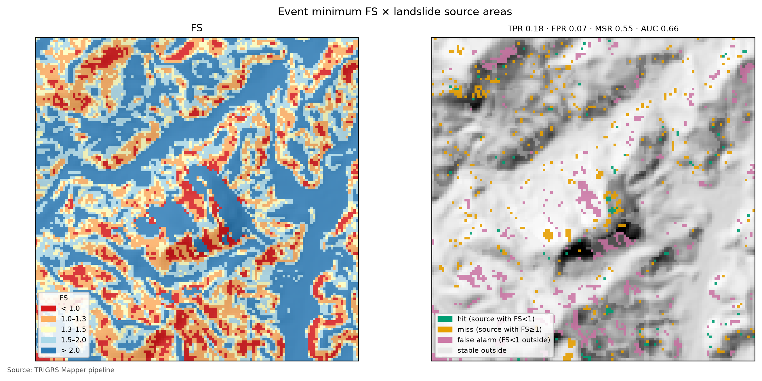
The ROC curve (Figure 6.36) does not depend on the FS = 1 threshold: ranking the cells from the lowest to the highest FS and sweeping the threshold, each value gives an (FPR, TPR) pair. The diagonal is chance (AUC = 0.5); the more the curve rises on the left, the better the FS ranks the cells, and the binary map (FS < 1) is a single point of this curve. Two configurations can have the same AUC and very different MSR — the AUC measures the ranking, the MSR the threshold —, and the AUC is little sensitive to the parameters (Seefelder and Mergili, 2016); this is why it enters only as a constraint. For the ensemble of the best samples, the score becomes the fraction of runs with FS < 1, which has few levels — hence the stepped curve.
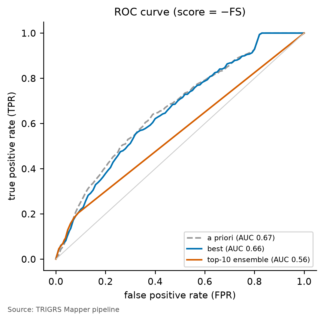
LRclass reads the same ranking through FS bands (Table 6.40). In the best sample, the FS < 1 class holds 17.8% of the source cells in 7.9% of the window (LR = 2.25; a priori, 0.91), and the 1 ≤ FS < 1.3 class, 29.9% of the source cells in 19.7% of the window (LR = 1.52). An LR that falls from the low-FS classes to the high-FS ones — as it should in a useful model — shows that the FS ranks the slopes even when the FS = 1 threshold misses many scars; classes just above 1 with LR > 1 reveal “nearly unstable” scars, which small changes in the parameters or in the rainfall would bring to FS < 1.
In the calibrated configuration, the LR falls monotonically from the FS < 1 class to the FS ≥ 2 class. In the a priori run, the scars also concentrate in the low-FS classes, but the highest LR lies in the 1.3 ≤ FS < 1.5 class (LR = 2.50), just above the threshold: the ranking already existed, and the calibration brings these slopes below FS = 1 — which is why the ROC curves of the two runs nearly coincide.
| FS class | A priori: area (%) | A priori: scars (%) | A priori: LR | Best (lhs_0019): area (%) | Best: scars (%) | Best: LR |
|---|---|---|---|---|---|---|
| FS < 1 | 0.6 | 0.6 | 0.91 | 7.9 | 17.8 | 2.25 |
| 1 ≤ FS < 1.3 | 3.6 | 8.0 | 2.24 | 19.7 | 29.9 | 1.52 |
| 1.3 ≤ FS < 1.5 | 7.4 | 18.6 | 2.50 | 13.4 | 14.2 | 1.06 |
| 1.5 ≤ FS < 2 | 27.0 | 34.3 | 1.27 | 21.5 | 18.4 | 0.85 |
| FS ≥ 2 | 61.4 | 38.6 | 0.63 | 37.5 | 19.7 | 0.53 |
ImportantThe FS does not rank the cells better than slope alone
A simple test puts the AUC in perspective: replace the −FS score with the slope, using the same positive and negative cells of the window. Slope alone has AUC = 0.70, against 0.66 for the calibrated FS; in Teresópolis, 0.85 vs. 0.76, and in Petrópolis, 0.58 vs. 0.58 (Chapters 7 and 8). The calibrated TRIGRS does not rank spatial susceptibility better than slope.
This is not a computational error but a consequence of the form of the FS. Slope enters it through several paths — in the friction term, tan φ′/tan δ, in the thickness zmax, which the model of Section 6.8.3 derives from slope itself, and in the initial water table, a fraction of zmax —, and what is left carries no spatial information that the scars confirm: the properties are constant within each zone, defined by simple rules on the DEM, the land cover, and maps at 1:100,000 to 1:250,000, the multipliers are the same over the whole window, and so is the rainfall. In Nova Friburgo, part of the difference comes from the outcrop: some 2011 source areas lie on the scarp, which is steep — slope places them at the top of the ranking — but is treated as rock that does not fail (Section 6.8.2). Even outside the outcrop, however, the FS does not beat slope.
What does this change in the use of TRIGRS? To say where failures may occur, slope does the same job with far fewer assumptions, and the FS map should not be presented as a susceptibility zoning better than slope. What slope does not provide, and TRIGRS does, is the when and the how much: which slopes a storm takes from FS ≥ 1 to FS < 1 — depending on the duration, the return period, the climate scenario, and the initial condition (the thresholds of Section 6.10.7) — and with what depth and volume (Section 6.10). This is where the value of the coupling with GIDES lies, and this is why the calibration is judged by \(MSR_{trig}\), which measures the timing, while the AUC enters only as a constraint. The D21 skill flag (Section 6.9.4) compares the model with chance, not with this baseline: it says that the configuration hits triggered failures better than chance, not that the FS map is better than the slope map.
6.9.6 Cross-validation
The validation question is practical: do the parameters calibrated in one watershed work in another, without recalibration? The Nova Friburgo multipliers were applied to the Teresópolis calibration window, with the 2011 rainfall and inventory of that case (Chapter 7), and compared with three references: the a priori run on the target, the best sample of the target’s own calibration, and the position of the Nova Friburgo configuration in the ranking of the target’s samples — possible because the sample design is the same in the three cases.
With the Nova Friburgo multipliers, the target — Teresópolis (calibration window) — has MSR = 0.56 (a priori: 0.53; difference of +0.039) and AUC = 0.76 (a priori: 0.79). The best sample of the Teresópolis calibration has MSR = 0.56, and the Nova Friburgo configuration ranks 38 of 150 in the Teresópolis ranking. By the D21 criterion, the transferred \(MSR_{trig}\) is 0.56 (a priori: 0.53; difference of +0.031), against 0.56 for the target’s own calibration, and its position in the Teresópolis ranking by \(MSR_{trig}\) is 21 of 150 (Table 6.41).
| Origin → target (rainfall) | Scars (source cells) | Transferred MSR | A priori MSR | Target MSR | Triggered MSR: transferred / a priori / target | AUC transferred / a priori | Rank in the target LHS (MSR; triggered MSR) |
|---|---|---|---|---|---|---|---|
| Nova Friburgo → Teresópolis (calibration window) (rainfall of Teresópolis) | 318 (647) | 0.56 | 0.53 | 0.56 | 0.56 / 0.53 / 0.56 | 0.76 / 0.79 | 38 of 150; 21 of 150 |
The transfer works. In Teresópolis, the Nova Friburgo multipliers beat the a priori run by both criteria — MSR (+0.039) and \(MSR_{trig}\) (+0.031) —, and the transferred \(MSR_{trig}\) equals that of the target’s own calibration. The reason is the most direct test that the shared sample design allows: the Teresópolis calibration, carried out independently, with other scars and another storm, picked the same sample, lhs_0019 (Chapter 7). The positions 38 of 150 (MSR) and 21 of 150 (\(MSR_{trig}\)) count all the Teresópolis samples: those ranked ahead of it were rejected by the selection of that case — almost all of them for leaving slopes unstable before the rain —, and, among the samples that pass the selection, the Nova Friburgo configuration ranks first by \(MSR_{trig}\). Only the AUC falls below that of the a priori run on the target (0.76 vs. 0.79), as in Nova Friburgo: the calibration moves the threshold, not the ranking (Section 6.9.5).
The calibration therefore captured something regional — the same material, the same kind of extreme rainfall, the same mechanism —, and not only the particulars of the Nova Friburgo window: for the 2011 event, there is a coherent parameter set for both watersheds. The test counts because it is independent: the two windows do not overlap, and each calibration uses its own scars and its own rainfall. But it is a single test, with a single event, and it does not extend by itself to other watersheds.
WarningThe Vale do Cuiabá is not a second independent validation
In the Petrópolis case study, the configuration chosen there is transferred to the Vale do Cuiabá, with the 2011 inventory. That window, however, covers 66.5% of the Teresópolis calibration window and 96.2% of the cells of the Teresópolis watershed, and it uses the 2011 Teresópolis rainfall: the fit there is, to a large extent, a fit in the Teresópolis area. The test validates neither Petrópolis nor the 2022 rainfall, and it does not allow attributing the lack of skill of that case to the preliminary 2022 inventory alone: with the 2022 rainfall, the model leaves 22.1% of the Petrópolis watershed unstable, where there are almost no scars — it overestimates the instability. This is why, in Petrópolis, the regional configuration (lhs_0019) enters only as a recommended sensitivity run, and the volumes remain a scenario.
6.9.7 Sensitivity
The sensitivity analysis varies one factor at a time around the calibrated configuration, in the 30 m window, and measures the effect on three things: the total hit rate (MSR and AUC in the window), the hit rate of the triggered failures (Δ triggered MSR), and the event volume on the watershed (Vdep of all unstable cells inside the watershed mask). The variations cover the weakest assumptions of the model:
- initial water table: \(d\) = 1 to 10 m (D6) and fractions 0.5, 0.75, and 1.0 of
zmax; - soil thickness:
zmaxfrom the DeRose curve, uniform at 1.25 and 2.0 m, linear, and from the rescaled BDTICM pattern; - strength: c′ × 0.5 and × 2; tan φ′ × 0.85 and × 1.15 (the limits of the hypercube ranges);
- hydraulics: Ks × 0.1 and × 10;
- event rainfall: the minimum, rain-gauge IDW, original MERGE, and maximum scaling scenarios (Table 6.20);
- runoff: the SCS-CN variant, in which only the P − Pe part of the rainfall infiltrates, with the CN of Section 6.5.6 (AMC II). It is built into the pipeline, but it only runs when the watershed CN is read from
chuva/cn.json, and the pipeline reader does not recognize the format of the Nova Friburgo file (one CN per moisture condition): the variant was not run and does not appear in Table 6.42, which lists the variations actually run; - model: saturated mode (no suction) and
flowdir=hydro(no drainage through the base); - resolution: the event on the watershed at 30 and at 10 m and the calibrated configuration checked on the window itself at 10 m (D12).
| Variation | Vdep (m³) | ΔVdep (%) | MSR | ΔMSR | Δ triggered MSR | AUC |
|---|---|---|---|---|---|---|
| base configuration | 17,138 | n/a | 0.55 | n/a | (0.54) | 0.66 |
| initial water table d = 1 m | 10,923 | −36.3 | 0.52 | −0.030 | −0.022 | 0.66 |
| initial water table d = 2 m | 3,493 | −79.6 | 0.50 | −0.051 | −0.042 | 0.67 |
| initial water table d = 3 m | 3,493 | −79.6 | 0.50 | −0.051 | −0.042 | 0.67 |
| initial water table d = 4 m | 3,493 | −79.6 | 0.50 | −0.051 | −0.042 | 0.67 |
| initial water table d = 5 m | 3,493 | −79.6 | 0.50 | −0.051 | −0.042 | 0.67 |
| initial water table d = 6 m | 3,493 | −79.6 | 0.50 | −0.051 | −0.042 | 0.67 |
| initial water table d = 7 m | 3,493 | −79.6 | 0.50 | −0.051 | −0.042 | 0.67 |
| initial water table d = 8 m | 3,493 | −79.6 | 0.50 | −0.051 | −0.042 | 0.67 |
| initial water table d = 9 m | 3,493 | −79.6 | 0.50 | −0.051 | −0.042 | 0.67 |
| initial water table d = 10 m | 3,493 | −79.6 | 0.50 | −0.051 | −0.042 | 0.67 |
| initial water table = 1·zmax | 3,493 | −79.6 | 0.50 | −0.051 | −0.042 | 0.67 |
| initial water table = 0.75·zmax | 9,731 | −43.2 | 0.51 | −0.038 | −0.030 | 0.66 |
| initial water table = 0.5·zmax | 17,138 | 0.0 | 0.55 | 0.000 | 0.000 | 0.66 |
| uniform zmax of 1.25 m | 14,438 | −15.8 | 0.54 | −0.016 | −0.014 | 0.66 |
| zmax: DeRose model | 10,358 | −39.6 | 0.52 | −0.028 | −0.022 | 0.65 |
| zmax: linear (4 → 0.3 m) model | 9,119 | −46.8 | 0.52 | −0.030 | −0.024 | 0.65 |
| uniform zmax of 2.0 m | 27,660 | +61.4 | 0.57 | +0.018 | −0.002 | 0.66 |
| zmax: regolith (BDTICM) model | 32,486 | +89.6 | 0.55 | −0.006 | −0.024 | 0.65 |
| Ks × 10 | 9,865 | −42.4 | 0.52 | −0.036 | −0.036 | 0.65 |
| Ks × 0.1 | 7,314 | −57.3 | 0.51 | −0.041 | −0.041 | 0.67 |
| c′ × 0.5 | 26,202 | +52.9 | 0.59 | +0.034 | +0.015 | 0.66 |
| c′ × 2 | 7,314 | −57.3 | 0.52 | −0.036 | −0.029 | 0.66 |
| tan φ′ × 0.85 | 23,704 | +38.3 | 0.56 | +0.007 | −0.006 | 0.66 |
| tan φ′ × 1.15 | 14,995 | −12.5 | 0.53 | −0.026 | −0.018 | 0.66 |
| event rainfall: maximum scenario | 18,265 | +6.6 | 0.55 | +0.001 | +0.001 | 0.66 |
| event rainfall: raw MERGE scenario | 18,265 | +6.6 | 0.55 | −0.002 | −0.002 | 0.66 |
| event rainfall: minimum scenario | 15,017 | −12.4 | 0.53 | −0.018 | −0.018 | 0.66 |
| event rainfall: rain gauges (IDW) scenario | 17,138 | 0.0 | 0.55 | +0.001 | +0.001 | 0.66 |
| saturated model | 18,265 | +6.6 | 0.55 | 0.000 | −0.009 | 0.65 |
| flowdir = hydro | 27,233 | +58.9 | 0.60 | +0.049 | +0.026 | 0.66 |
| watershed resolution 10 m × 30 m — all unstable cells | 17,017 (30 m: 17,138) | −0.7 | n/a | n/a | n/a | n/a |
| watershed resolution 10 m × 30 m — patch (D19 total, incl. FS0 < 1) | 1,392 (30 m: 3,493) | −60.1 | n/a | n/a | n/a | n/a |
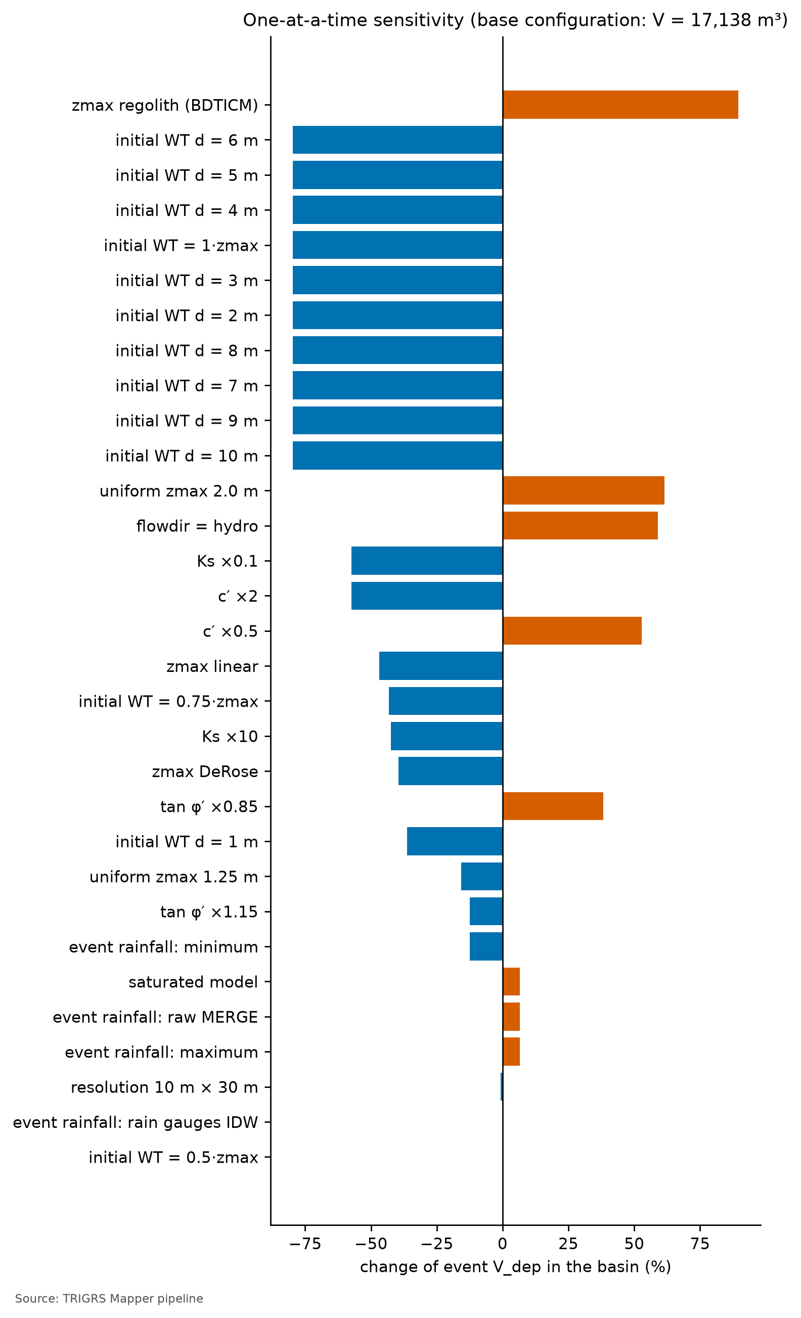
The factor with the largest effect on the event Vdep is zmax: regolith (BDTICM) model (+89.6%), and the one with the largest effect on the MSR, initial water table = 1·zmax (−0.051), tied with all the fixed water tables from 2 to 10 m. With the initial water table at 1 m, Vdep changes by −36.3%; with the water table at 10 m — at the soil base —, by −79.6%. In the base configuration, the \(MSR_{trig}\) in the window is 0.54 (total MSR: 0.55). The largest effects on the volume come from the two assumptions with no measurements in the watershed — the soil thickness and the initial water table —, and the physics helps to read the tornado:
- Initial water table. A shallow water table imposes positive pressure at the base from the start and lowers the FS even before the rain; it is usually the dominant hydrological factor (Zieher et al., 2017). Here the effect goes one way only: on the slopes that fail, the calibrated water table, at mid-thickness, is the wettest condition of the tornado, and all the others — water table at 1 m, at 0.75 of the thickness, or at the base — reduce the volume, the MSR, and \(MSR_{trig}\). From \(d\) = 2 m on, the result is the same as with the water table at the base, because, with the calibrated \(m_z\), the slopes that fail have
zmaxbelow 2 m. A shallow water table can also create cells with \(FS_0 < 1\): compare, in Table 6.42, the ΔMSR and Δ triggered MSR columns — a variation that raises the total MSR and lowers the triggered one gains hits from the initial condition, not from the rainfall. - Soil thickness. The two largest volume increases come from swapping the
zmaxmodel — the rescaled BDTICM pattern (+89.6%) and the uniform 2.0 m thickness, thicker than the calibrated one on the slopes that fail (+61.4%); the other three forms (DeRose, linear, and uniform 1.25 m) reduce the volume. This is expected, because failure always occurs at the base of the soil and the volume per cell is the area times the thickness itself (Section 6.10.4). The larger volume does not come with triggered hits: \(MSR_{trig}\) does not improve in either of the two. Thickness is, together with the initial water table, the assumption with the largest effect — and the weakest one in the model (box in Section 6.8.3). - c′ and tan φ′. Cohesion weighs more in shallow soils, because its term, \(c'/(\gamma_s Z \sin\delta\cos\delta)\), grows as Z decreases (Chapter 1); tan φ′ multiplies both friction and the effect of pore pressure. Lowering the strength increases the volume and the total MSR, but the gain in \(MSR_{trig}\) is much smaller — with tan φ′ × 0.85, \(MSR_{trig}\) even drops —: part of the new hits were already unstable before the rain.
- Ks. It acts both ways: a higher Ks lets more rain infiltrate and carries the pressure front faster to the base; a lower Ks generates more runoff and delays the response. Both variations — × 0.1 and × 10 — reduce the volume and the MSR, and \(MSR_{trig}\) drops as much as the total MSR: the calibrated Ks is close to the best value for the event, and the whole effect is on triggered failures.
- Model. The saturated mode, without suction, barely changes the volume (+6.6%) and the MSR (0.000). By contrast,
flowdir=hydro— in TRIGRS, a hydrostatic initial pressure and no drainage through the base — increases the volume (+58.9%) and gives the largest MSR gain of the tornado (+0.049; \(MSR_{trig}\): +0.026). Retaining water at the base improves the fit, which is consistent with the perched water table described for 2011 (Section 6.8.5). Since it is a variation around a configuration calibrated withgener, it does not replace the calibration; it suggests testinghydroin the search itself (Section 6.11.3). - Event rainfall. The scaling scenarios change the volume little — −12.4% for the minimum, 0.0% with the rain-gauge IDW, +6.6% with the original MERGE, and +6.6% for the maximum — and \(MSR_{trig}\) (−0.018 for the minimum and +0.001 for the maximum). The response is asymmetric: reducing the rain removes more instability than increasing it adds, and the original MERGE and the maximum scenario, with much more rain than the central one, give the same volume. The initial condition is not what decides — only 8.5% of the event’s unstable cells were already unstable before the rain —: the 2011 rainfall lies far above the thresholds of the watershed (Section 6.10.7), and the response saturates. The uncertainty in the event rainfall weighs much less than that of the parameters.
Resolution. The resolution runs use the controls of the calibration phase (Section 6.8.6: nzs = 20, a minimum slope of 10°, and only the four calibration outputs) and therefore differ slightly from the final event run on the watershed (Section 6.10.4). At 10 m, the Vdep of all unstable cells of the event on the watershed is 17,017 m³, against 17,138 m³ at 30 m (−0.7%); the unstable fraction is 14.0% vs. 11.6%. The Vdep of the patch connected to the drainage is 1,392 m³ at 10 m and 3,493 m³ at 30 m (−60.1%) and accounts for 8.2% of the Vdep of all unstable cells at 10 m and for 20.4% at 30 m (Section 6.10.3). The resolution barely changes the volume of all unstable cells, and the unstable fraction rises a little at 10 m; what changes is the connection to the drainage: at 10 m, the channels are narrower, and the connected patch loses more than half of its volume. The calibrated configuration was also checked on the window itself at 10 m: MSR of 0.54 (at 30 m, 0.55), \(MSR_{trig}\) of 0.53 (at 30 m, 0.54), and AUC of 0.68 (at 30 m, 0.66). The scores barely change: transferring the multipliers from the 30 m window to the 10 m grid (D12) does not lose skill. The unstable area, however, does change: at 10 m, the set calibrated at 30 m leaves 6.0% of the window unstable, against 7.9% at 30 m — the MSR can stay almost the same with fewer unstable cells because, at 10 m, the model loses hits and false alarms at the same time. The multipliers are therefore not neutral to resolution, and the effect does not even have the same sign everywhere: on the window, the unstable fraction drops at 10 m; on the watershed, it rises. The volumes of the 10 m watershed inherit this uncertainty, and the Teresópolis and Petrópolis windows show the same drop (at 10 m vs. at 30 m: 2.6% vs. 4.7% and 14.8% vs. 20.6%).
6.9.8 What the calibration teaches
- A modest gain, but from the rainfall. \(MSR_{trig}\) went from 0.50 (a priori) to 0.54, and the total MSR from 0.50 to 0.55. An MSR close to 0.5 is chance performance, and the a priori run, with the water table at the base, has almost no unstable cells. The gain is small, but it comes from failures triggered by the rainfall, and the configuration passes the skill criterion: minimum skill met (triggered TSS 0.09 ≥ 0.05 and AUC 0.66 ≥ 0.60).
- Timing matters. Under the total MSR, the choice would fall on a sample whose hits come from slopes already unstable before the rain. The chosen sample has 0.67% of the window unstable before the event, and only 8.5% of its unstable cells in the event already were: the instability it produces is triggered by the rainfall.
- The AUC does not discriminate. With the AUC of the samples in a narrow band (0.65–0.67), the AUC ≥ 0.70 constraint is not attainable, and the calibration does not improve on the AUC of the a priori run: it shifts the FS = 1 threshold without changing how the slopes are ranked (Figure 6.36 and Table 6.40). And slope alone ranks the cells better than the calibrated FS (AUC of 0.70 vs. 0.66): what TRIGRS adds is not the map of where failures occur, but the timing of the failure and the volume (box in Section 6.9.5).
- Parameters at the limit. Several calibrated multipliers sit next to the edges of their ranges (Table 6.36): \(m_z\) (0.62) at the lower bound — soils thinner than the a priori ones —, \(m_{Cr}\) (1.42) near the upper bound, \(m_\alpha\) (0.57) and
rizero(1.47 × 10⁻⁹ m/s) near the lower bound, and \(f_{NA}\) = 0.50, the shallowest of the three allowed water tables. When the optimum touches the edges, the a priori range may be constraining the search — or the model may be compensating for another simplification, such as the lack of lateral flow. Thin soil, strong roots, and a wet start together leave the slopes standing, but close to the threshold, before the rain: this is what the selection requires and what the thresholds show (Section 6.10.7). The calibrated \(f_{NA}\) is an effective parameter (Section 6.8.4). - Winner vs. ensemble. The 1st and 2nd samples differ by 0.006 in \(MSR_{trig}\): read the top three and the ensemble, not just the winner.
- A regional configuration. The Teresópolis calibration picked the same sample, and the transfer improves on the a priori run in that case (Section 6.9.6); on the window itself at 10 m, the scores barely change, although the unstable area drops from 7.9% to 6.0% (Section 6.9.7). For the 2011 event, there is a coherent parameter set for both watersheds. It is a single test, with one event; the transfer to the Vale do Cuiabá, in Chapter 8, is not a second one, because it largely repeats the area and the rainfall of Teresópolis.
- Limits of the test. A regional inventory that does not separate failure from deposit, a 30 m DEM that postdates the event, and a reconstructed storm limit the cell-by-cell accuracy that can be achieved; this is why we also look at the scar detection rate, at LRclass, and at the patterns of the map.
6.10 From TRIGRS to Vdy12
With the calibrated configuration, TRIGRS runs on the 10 m watershed for the 2011 event and for the design storms. This section turns the unstable cells into a volume and fits this volume into the GIDES accounting of Section 6.7 — the physically based Vdy12 announced at the end of that section.
6.10.1 Three forms of volume (decision D18)
In an unstable cell, the material above the failure surface is a prism of area \(A_{px}\) and height \(Z_{cr}\). Since TRIGRS measures Z vertically, the volume of this prism is exactly \(A_{px}\,Z_{cr}\) (the slope-normal thickness, \(Z_{cr}\cos\delta\), times the inclined area, \(A_{px}/\cos\delta\)). The sum over the unstable cells can be expressed on three bases:
\[ \begin{aligned} V_{insitu} &= \sum_{FS_i<1} A_{px}\,Z_{cr,i},\\ V_{dep} &= \sum_{FS_i<1} A_{px}\,Z_{cr,i}\,\frac{1-\theta_{s,i}}{1-\lambda},\\ V_{solto} &= \frac{V_{insitu}}{1-\lambda}, \qquad \lambda = 0.4. \end{aligned} \]
- Vinsitu is the soil as it stands on the slope, with its voids. It is directly comparable to the manual’s Vdy11 and Vdy12, which are also in situ volumes — widths, depths, and lengths measured in the field —, with bulking neglected (BRASIL/MI; JICA, 2018; NILIM, 2016a).
- Vdep converts this soil into a deposit through the conservation of solids. The volume of grains does not change when the soil fails and is deposited: \(V_{insitu}\,(1 - n_s) = V_{dep}\,(1 - \lambda)\), where \(n_s \approx \theta_s\) is the porosity of the in situ soil (the \(\theta_s\) of the zone) and λ = 0.4 is the porosity of the deposit — the same constant \(K_v\) as in Equation 6 for Vdy2. It is the main form (D18) and the basis of Vdy12*.
- Vsolto (bulked volume) applies 1/(1 − λ) to the in situ volume as if the soil column had no voids: it is an upper bound, 67% above Vinsitu.
NoteWhy Chapter 5 used Vsolto
In the tutorial example (Section 5.7), the in situ volume was divided by (1 − λ) to put it “on the same basis as the manual”, which works with the deposited sediment, with voids. The reasoning assumes that the intact soil has no voids — but the hillslope soil already has 38 to 50% voids (the \(\theta_s\) values of Table 6.29). Counting the voids on both sides, the factor becomes \((1-\theta_s)/(1-\lambda)\), close to 1 when the porosity of the soil is similar to that of the deposit. The Chapter 5 procedure remains valid as an illustration of the method; in the case studies, we adopt Vdep as the main form and keep Vsolto as a ceiling (decision D18).
6.10.2 Worked example: from one cell to the volume
Consider a 10 m cell (Apx = 100 m²) of colluvium (\(\theta_s\) = 0.48) that becomes unstable with \(Z_{cr}\) = 1.6 m (illustrative values):
- \(V_{insitu} = 100 \times 1.6 = 160\) m³ — the soil prism as it stands on the slope;
- \(V_{dep} = 160 \times (1 - 0.48)/(1 - 0.4) = 160 \times 0.867 \approx 139\) m³ — the same volume of grains, deposited with 40% voids;
- \(V_{solto} = 160/(1 - 0.4) \approx 267\) m³ — the ceiling, as if the slope had no voids.
Table 6.43 generalizes the conversion to the units of the watershed. Since the residual soil (\(\theta_s\) = 0.50) covers most of the soil area (Table 6.30), Vdep is close to 0.85 of Vinsitu, and Vsolto close to twice Vdep.
| Unit (\(\theta_s\)) | Vdep/Vinsitu = (1 − θs)/(1 − λ) | Vsolto/Vinsitu = 1/(1 − λ) |
|---|---|---|
| colluvium (0.48) | 0.87 | 1.67 |
| mature residual soil (0.50) | 0.83 | 1.67 |
| shallow soil over rock (0.45) | 0.92 | 1.67 |
| talus/alluvial deposit (0.38) | 1.03 | 1.67 |
D18/D19 volumes of a run with trigrs_mapper (excerpt)
import numpy as np
from trigrs_mapper.trigrs.volume import calcular_volume_trigrs

r = np.load("data/cases/nova_friburgo/runs/projeto/tr100_presente_atual_obs/resultado.npz")
for conect in ("todas", "mancha", "trajetoria"):   # all, patch, path
    v = calcular_volume_trigrs(r["fs_min"], r["zcr_fs_min"], area_celula=100.0, mascara_bacia=bacia,
                               lambda_porosidade=0.4, porosidade_solo=theta_s,  # θs of the zone, cell by cell
                               conectividade=conect, drenagem=canal, direcoes=d8_topoindex)
    print(conect, round(v.v_insitu_m3), round(v.v_dep_m3), round(v.v_solto_m3))
6.10.3 Which cells feed the debris flow: connectivity (decision D19)
Not all soil that fails becomes debris flow at the reference point. The manual defines Vdy1 as the sediment that can be “converted into debris flow” (BRASIL/MI; JICA, 2018, §2.5.1.1) — the material that reaches the channel. An isolated failure high on a convex slope may stop on the slope itself. Since TRIGRS does not model runout, we use three criteria of connectivity with the drainage network — the channels with A ≥ 1 ha of Section 6.4 —, illustrated in Figure 6.38:
- all (todas): any unstable cell of the watershed counts. It is the literal reading of the manual’s method “a” (all slopes that can fail) and the upper bound;
- patch (mancha): the patches of unstable cells (8-cell neighborhood) that contain or touch a channel cell count. It is the main criterion: Vdy12* is the Vdep of the patch (decision D19), formed, since D21, only by the cells triggered by the rainfall (see below);
- path (trajetória): only the cells whose D8 path to the channel passes exclusively through unstable cells count. It is the lower bound.
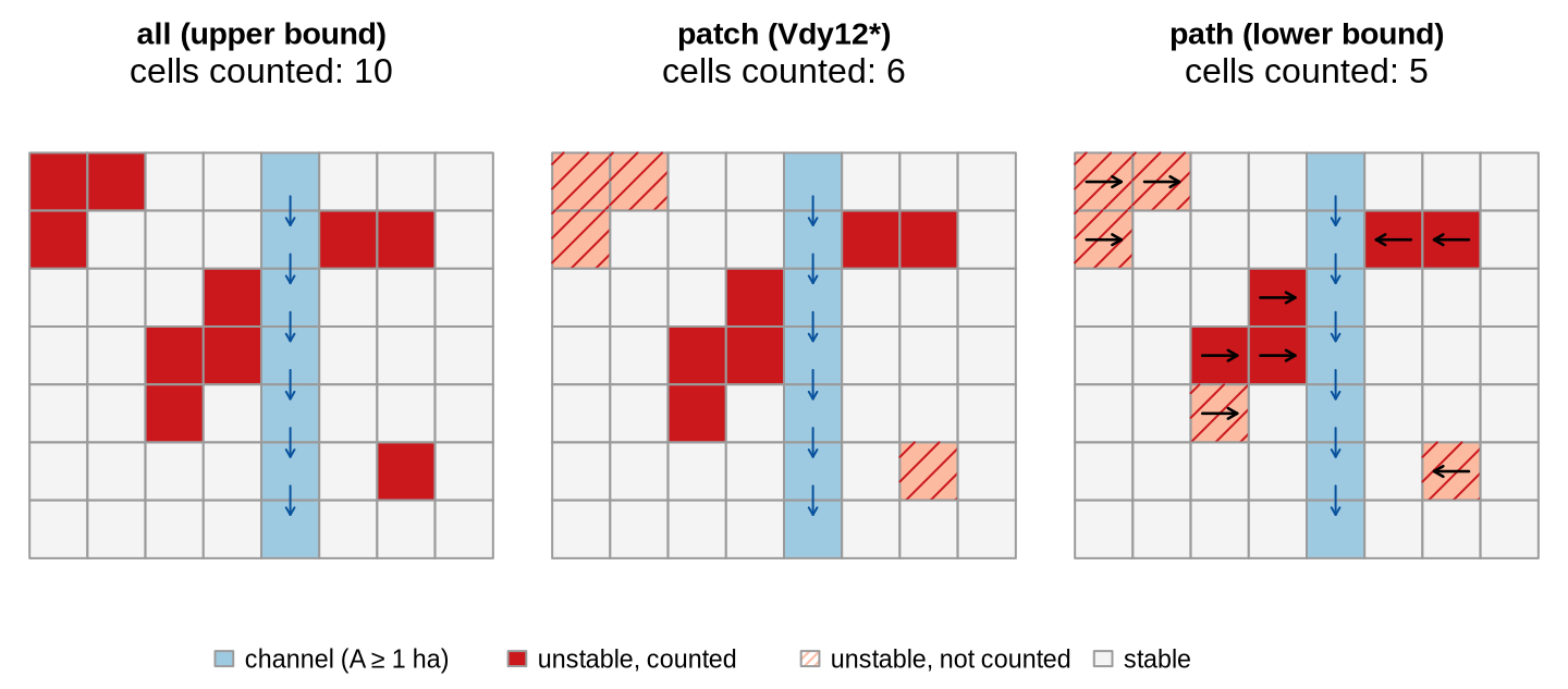
Connectivity depends on resolution: at 30 m, a single unstable cell next to the channel connects large patches; at 10 m, the channels are narrower and the patches more fragmented. In the reduced test of Petrópolis, the patch was about 7% of all unstable cells at 10 m and about 90% at 30 m (D19); in Nova Friburgo, in the 2011 event, 8.2% at 10 m and 20.4% at 30 m (resolution runs of Section 6.9.7; in the final event run, 7.4% at 10 m). That is why Vdy12* is always reported on the 10 m watershed, next to the two bounds.
Triggered cells vs. initial condition (decision D21). With the FS0 of each cell (Section 6.8.4), each volume is computed in three variants:
- triggered (
_defl): only the cells with \(FS_0 \ge 1\) and minimum FS < 1. The patches and the paths are formed by these cells only — the cells already unstable at t = 0 count as stable and break the connection; - total (no suffix; the D19 Vdy12*): all unstable cells, including those with \(FS_0 < 1\);
- initial (
_inicial): only the cells with \(FS_0 < 1\), with the \(Z_{cr}\) of the run.
Vdy12* is the Vdep of the triggered patch (pipeline.volumes.principal: dep_mancha_defl): what the design rainfall makes unstable and reaches the drainage network. The D19 total is kept as a conservative upper bound, and the initial share is reported separately, because it responds neither to the return period nor to the climate. For todas (all cells), total = triggered + initial; for the patch and the path, it is not: since the connection changes when part of the cells drops out, the total can exceed the sum of the other two. With few cells with \(FS_0 < 1\) — which the calibration filters ensure —, the difference is small.
Triggered Vdy12* of a run (excerpt; same logic as pipeline/projeto.py)
import numpy as np
from trigrs_mapper.trigrs.fs_inicial import condicao_inicial

ci = condicao_inicial(dom, par, cfg, "final")      # FS0 and Z_cr0 at t = 0, without running TRIGRS (D21)
ini = ci.instavel()                                 # FS0 < 1: already unstable at the initial condition
fs_defl = np.where(ini, np.inf, r["fs_min"])        # triggered cells only; the initial ones count as stable
v = calcular_volume_trigrs(fs_defl, r["zcr_fs_min"], area_celula=100.0, mascara_bacia=bacia,
                           lambda_porosidade=0.4, porosidade_solo=theta_s,
                           conectividade="mancha", drenagem=canal)
print("Vdy12* =", round(v.v_dep_m3), "m³")          # V_dep of the triggered patch
6.10.4 The 2011 event on the watershed: Zcr and volume by cell
With the calibrated configuration and the event rainfall, 171 cells of 10 m become unstable in the watershed — 1.71 ha, 15.2% of the area —, with a mean \(Z_{cr}\) of 1.31 m. Of these, 166 are triggered by the rainfall (14.8% of the watershed), and 2.9% of the unstable cells were already unstable at t = 0. At the initial condition of the event (2010 land cover), \(FS_0 < 1\) in 5 cells (0.44% of the watershed), and the state at t = 0 has a patch Vdep (V0) of 203 m³.
Table 6.44 crosses the three volume forms with the three connectivities, for the triggered cells only and for the total. The event Vdy12* is 1,189 m³ (Vdep of the patch connected to the drainage, with the rainfall-triggered cells only (D21)); the upper bound, the D19 total, is 1,392 m³, and the initial share accounts for 14.6% of it (Vdep of the patch formed only by the cells with \(FS_0 < 1\): 203 m³). In the total, the connected patch accounts for 7.4% of the Vdep of all unstable cells.
| Connectivity | Vinsitu triggered (m³) | Vinsitu total (m³) | Vdep triggered (m³) | Vdep total (m³) | Vsolto triggered (m³) | Vsolto total (m³) |
|---|---|---|---|---|---|---|
| all (upper bound) | 21,865 |
22,473 |
18,263 |
18,790 |
36,441 |
37,454 |
| patch (Vdy12*) | 1,399 |
1,634 |
1,189 | 1,392 |
2,332 |
2,723 |
| path (lower bound) | 472 |
707 |
412 |
615 |
787 |
1,178 |
How to compare with 2011? The São Lucas Hospital flow started from a planar failure in rock, in a stress-relief fracture zone high on the scarp (Section 6.1). This mechanism is beyond the reach of TRIGRS: on the scarp, the model sees outcrop, which does not fail. What TRIGRS estimates is the contribution of the soil-mantled slopes — colluvium, residual soil, and shallow soil. The comparison with the Vdy12 from method “a”, computed with the failure areas of the 2011 scars (Table 6.24), must keep this in mind: the source areas of the scars include stretches of the scarp that TRIGRS treats as rock.
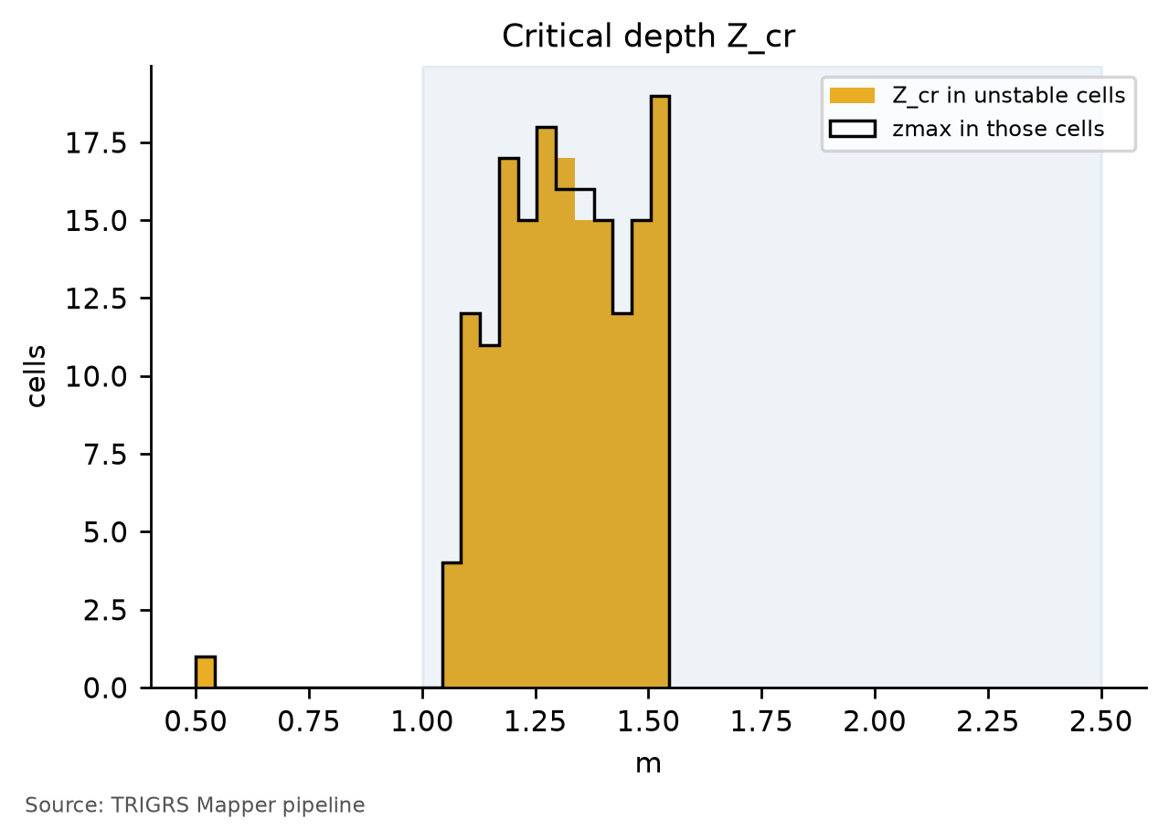
zmax (outline) in the unstable cells of the event, 10 m watershed. The shaded band (1–2.5 m) is that of the failures observed in the region. When the two histograms coincide, failure occurs at the base of the soil, at the less permeable contact — the mechanism described for 2011 (Marques et al., 2017; Machado, 2016); a bar at 0.5 m corresponds to the strip of shallow soil around the outcrop, whose zmax has this cap.
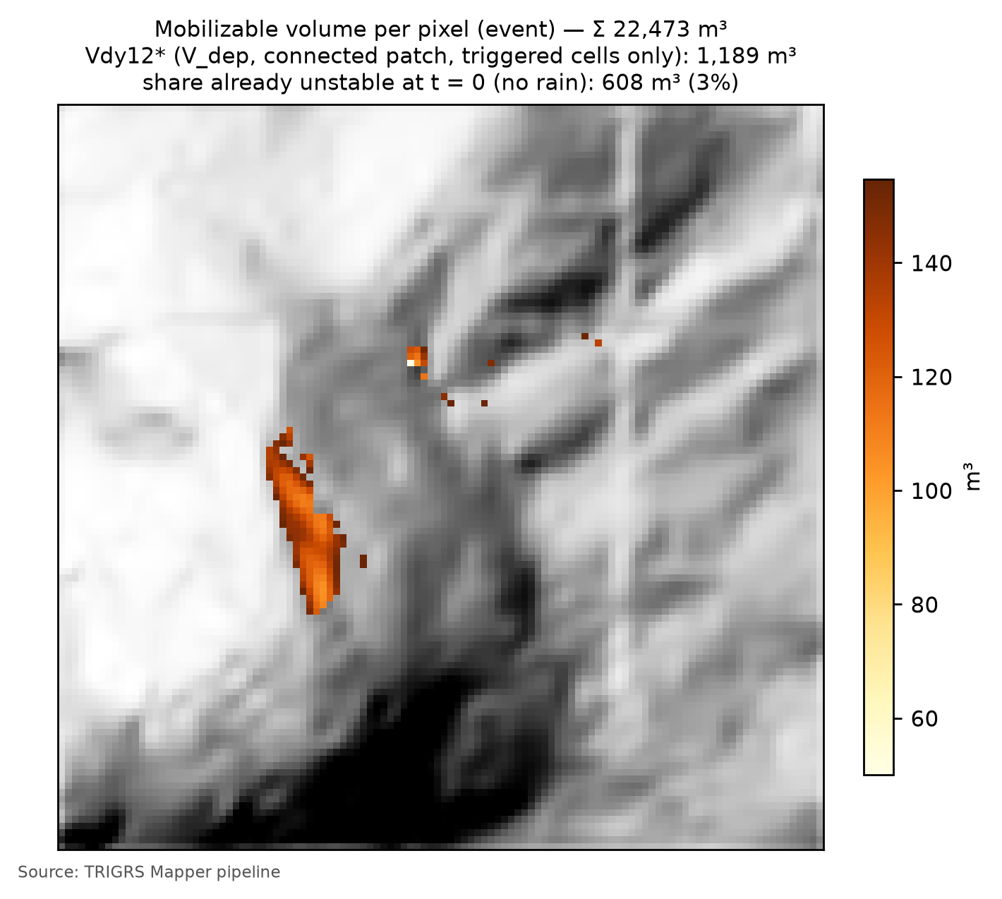
What the event shows. Almost all the instability of the event on the watershed is triggered by the rainfall: only 5 cells have \(FS_0 < 1\). Some of them, however, lie in patches connected to the drainage, and the initial share of Vdy12* exceeds 10% (14.6%): the upper bound (1,392 m³) should be read next to Vdy12* (1,189 m³).
Against method “a” (Table 6.24), TRIGRS gets right the order of magnitude of what fails, but not that of Vdy12. The unstable area of the event (1.71 ha) is of the order of the failure areas of the five scars inside the watershed, and the Vinsitu of all unstable cells (22,473 m³) falls within the range of method “a”, close to its central value. Vdy12*, however, counts only the patch connected to the drainage — 7.4% of the Vdep of all unstable cells — and stays an order of magnitude below method “a”. The difference between the two lies not in how much fails, but in how much reaches the channel: method “a” assumes that all the material of the failures becomes debris flow, whereas Vdy12* requires a connection to the drainage, which is narrow at 10 m (Section 6.10.3).
The two histograms of Figure 6.39 coincide: \(Z_{cr}\) = zmax in 100.0% of the unstable cells of the event on the watershed and in 100.0% of the unstable cells of the calibration window — as on the Teresópolis and Petrópolis watersheds (100.0% and 100.0%). Failure occurs at the base of the soil, at the less permeable contact — the mechanism described for 2011 —, with a mean \(Z_{cr}\) of 1.31 m, in the lower half of the 1–2.5 m range of the observed failures; only isolated cells sit at the 0.5 m cap of the shallow-soil strip. The failure depth is therefore the calibrated thickness itself: with \(m_z\) at the lower bound of its range, the volume per cell depends directly on a thickness that was not measured.
ImportantZcr = zmax: the volume comes from the thickness model
When the minimum FS always lies at the base of the profile, the volume computation simplifies: in an unstable cell, \(V_{insitu} = A_{px}\,Z_{cr} = A_{px}\,z_{max}\). The rainfall and the parameters decide which cells fail and when; how much each one delivers is the thickness given by the model of Section 6.8.3, that is, by slope and by the calibrated coefficients \(m_z\) and \(k_z\). Three consequences follow:
- Vdy12* inherits the
zmaxmodel. The volumes of this chapter — event, design, and Vd* — carry the uncertainty of a thickness derived from slope alone, the weakest option in Segoni et al. (2012) (box in Section 6.8.3). - The tornado shows the same. The two largest volume increases in the sensitivity analysis come from swapping the
zmaxmodel (Section 6.9.7): changing the thickness directly changes the volume of each cell that fails — and also which cells fail. - The median \(Z_{cr}\) tests the thickness, not the hydrology. The constraint of a median \(Z_{cr}\) between 1 and 2.5 m (Section 6.9.4) checks whether the coefficients \(m_z\) and \(k_z\) give the slopes that fail the thickness of the observed failures; it does not say whether the pressure front reaches the right depth. Measuring soil thickness is therefore the most direct way to constrain Vdy12* (Section 6.11.3).
6.10.5 Volume × return period, in the present and in the future
The design runs apply the 24-h hyetographs of Section 6.5.5 — 8 return periods (2 to 500 years) × 11 scenarios: the present; SSP2-4.5 and SSP5-8.5 in 2041–2070 (P50) and in 2071–2100 (P10, P50, and P90); SSP1-2.6 and SSP3-7.0 in 2071–2100 (P50) —, followed by 24 h without rain, on the MapBiomas 2025 land cover and with the calibrated configuration, including the initial condition (Section 6.8.4). The future hyetographs are the present ones multiplied by the change factor of each return period (Section 6.6). In each run, the FS of each cell is the minimum over time, and the volumes are summed in the three forms and the three connectivities, with the triggered cells only and with the total.
In the present, Vdy12* is the same for T = 25, 100, and 200 years — 1,382, 1,382, and 1,382 m³ —, even though the 24-h rainfall grows from 153.4 to 194.3 and 217.8 mm. For T = 100 years, the upper bound — the D19 total, with the cells already unstable at t = 0 — is 1,572 m³; the connectivity bounds range from 666 m³ (path, triggered cells only) to 14,709 m³ (all unstable cells); and 13.2% of the watershed becomes unstable, 12.7% through triggered cells. At the end of the century (2071–2100, P50), the 100-year Vdy12* stays at 1,382 m³ under SSP2-4.5 (0.0%; rainfall of 224.3 mm) and at 1,382 m³ under SSP5-8.5 (0.0%; rainfall of 260.7 mm), even though the unstable fraction of the watershed reaches 15.8%; for the upper bound, the change under SSP5-8.5 is 0.0%. Table 6.45 lists all the scenarios run — including P10, P90, SSP1-2.6, and SSP3-7.0 — and Figure 6.41 shows the curves.
The initial condition in the design runs. With the design land cover, \(FS_0 < 1\) in 5 cells of the watershed (0.44%; 1 of them unstable even without pore pressure), against 0.44% with the event land cover. The state at t = 0 has V0 = 190 m³ (patch Vdep; 513 m³ over all cells), the same for all return periods and scenarios. For T = 100 years in the present, 3.4% of the unstable cells were already unstable at t = 0, and 14.9% are already unstable at the first output of the run (≈ 2 h of rain), with a patch Vdep of 511 m³ at that moment. The initial share of Vdy12* for T = 100 years in the present, 1 − Vdy12* ÷ total, is 12.1%. Three flags summarize the initial condition (decision D21):
- relevant initial share (above 10%; the upper bound must be read next to Vdy12*): yes;
- consistency with the calibration (\(FS_0 < 1\) in more than 1% of the watershed with the event land cover): no;
- land-use effect (\(FS_0 < 1\) larger with the design land cover than with the event land cover — weaker slopes today, not a calibration error): no.
| Scenario / RP (yr) | 2 | 5 | 10 | 25 | 50 | 100 | 200 | 500 |
|---|---|---|---|---|---|---|---|---|
| present — path, triggered cells only (lower bound) | 533 | 533 | 666 | 666 | 666 | 666 | 666 | 666 |
| present — Vdy12* (patch, triggered cells only) | 1,249 | 1,249 | 1,382 | 1,382 | 1,382 | 1,382 | 1,382 | 1,382 |
| present — patch including cells unstable at t = 0 (D19 total; upper bound) | 1,439 | 1,439 | 1,572 | 1,572 | 1,572 | 1,572 | 1,572 | 1,572 |
| present — initial share (patch of the cells with FS0 < 1) | 190 | 190 | 190 | 190 | 190 | 190 | 190 | 190 |
| present — all unstable cells (literal reading of method a) | 6,995 | 9,437 | 10,667 | 12,241 | 12,930 | 14,709 | 16,175 | 18,035 |
| SSP1-2.6 2071–2100 P50 | 1,249 | 1,382 | 1,382 | 1,382 | 1,382 | 1,382 | 1,382 | 1,382 |
| SSP2-4.5 2041–2070 P50 | 1,249 | 1,382 | 1,382 | 1,382 | 1,382 | 1,382 | 1,382 | 1,382 |
| SSP2-4.5 2071–2100 P50 | 1,249 | 1,382 | 1,382 | 1,382 | 1,382 | 1,382 | 1,382 | 1,382 |
| SSP2-4.5 2071–2100 P10 | 1,249 | 1,382 | 1,382 | 1,382 | 1,382 | 1,382 | 1,382 | 1,382 |
| SSP2-4.5 2071–2100 P90 | 1,249 | 1,382 | 1,382 | 1,382 | 1,382 | 1,382 | 1,382 | 1,382 |
| SSP3-7.0 2071–2100 P50 | 1,249 | 1,382 | 1,382 | 1,382 | 1,382 | 1,382 | 1,382 | 1,382 |
| SSP5-8.5 2041–2070 P50 | 1,249 | 1,382 | 1,382 | 1,382 | 1,382 | 1,382 | 1,382 | 1,382 |
| SSP5-8.5 2071–2100 P50 | 1,249 | 1,382 | 1,382 | 1,382 | 1,382 | 1,382 | 1,382 | 1,382 |
| SSP5-8.5 2071–2100 P10 | 1,249 | 1,382 | 1,382 | 1,382 | 1,382 | 1,382 | 1,382 | 1,382 |
| SSP5-8.5 2071–2100 P90 | 1,382 | 1,382 | 1,382 | 1,382 | 1,382 | 1,382 | 1,382 | 1,382 |
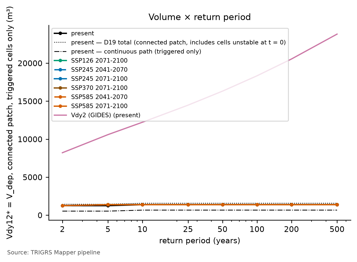
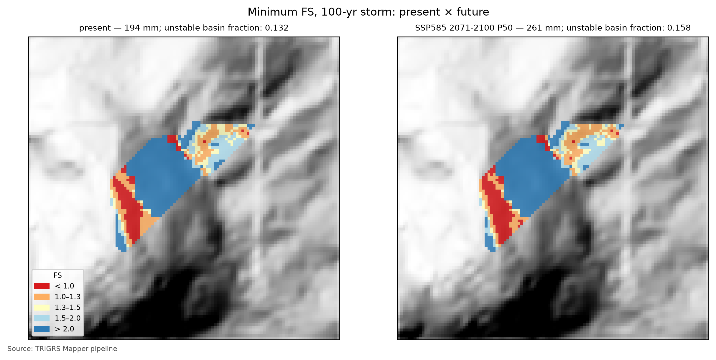
TipHow to read the volume curves
- The P10–P90 range is the spread across climate models, not a confidence interval (Section 6.6).
- A rising curve indicates that larger storms trigger new slopes: the volume responds to the return period and to the climate.
- A flat curve indicates that the unstable area is already set at the low return periods — the slopes that can fail already do. Before D21, a flat curve could hide something else: a Vdy12* dominated by the V0 of the initial condition, which responds neither to the return period nor to the climate. That share is now left out of Vdy12* and shows up in the upper bound: if the total is flat and the triggered volume rises, it was the initial condition that flattened the curve.
- Always compare with Vdy2 (pink line), which grows in the same proportion as the daily rainfall.
Flat curves: the connected patch saturates. In Nova Friburgo, Vdy12* barely responds to the return period or to the climate. In the present, it is 1,249 m³ for T = 2 and 5 years and 1,382 m³ from T = 10 to 500 years; in the future scenarios, the plateau arrives one return period earlier — at T = 5 years, or already at T = 2 years under SSP5-8.5 P90 —, and this earlier arrival is the only response to the climate (+10.6% for T = 5 years under SSP5-8.5 P50; no change from T = 10 years on). This is why the P10–P90 range practically vanishes and the SSP1-2.6 and SSP3-7.0 scenarios coincide with the others. The upper bound is equally flat — it is Vdy12* plus the V0 of 190 m³ —, so it is not the initial condition that flattens the curve (box above). The watershed, however, becomes increasingly unstable: the unstable fraction goes from 7.0% for T = 2 years to 15.6% for T = 500 years in the present (and to 18.5% under SSP5-8.5 P90), and the Vdep of all unstable cells grows from 6,995 to 18,035 m³. The cells that the larger storms add form patches that do not touch the drainage: at 10 m, whatever can fail next to the channel already fails with the 10-year storm, and Vdy12* has nowhere left to grow.
Initial-condition flags. With the design land cover, only 5 cells have \(FS_0 < 1\) (0.44% of the watershed), the same fraction as with the event land cover: there is no land-use effect, and the initial condition is consistent with the calibration, well below 1%. Some of these cells, however, lie in patches connected to the drainage, and the initial share of Vdy12* for T = 100 years in the present (12.1%) exceeds 10%: the relevant-share flag is on, and the upper bound must be read next to Vdy12*. The difference between the two is V0, the same for all return periods and scenarios.
6.10.6 From Vdy12* to the design volume (Vd*)
Vdy12* replaces the traditional Vdy12 in the manual’s rule:
\[ \begin{aligned} V_{dy1}^{*} &= V_{dy11} + V_{dy12}^{*},\\ V_d^{*} &= \max\left[\min\left(V_{dy1}^{*},\, V_{dy2}\right),\ 1{,}000\ \text{m}^3\right],\\ V_{plano}^{*} &= V_d^{*} + V_{wy}. \end{aligned} \]
Vdy11 (channel bed, orders ≥ 1) remains that of Section 6.7 — 5,886 m³ —, because TRIGRS does not model the channel bed; the Vdy2 of each return period and scenario comes from Table 6.25 and Table 6.26, and the woody debris adds Vwy = 58 m³ (Table 6.46). With the upper bound of Vdy12* in place of the main value, the same equations give the conservative Vd*, which the table shows in parentheses.
| Scenario | RP (yr) | Vdy12* (upper bound) (m³) | Initial share (%) | Vdy1* (m³) | Vdy2 (m³) | Vd* (upper bound) (m³) | Governs | Trad. Vd (governs) (m³) |
|---|---|---|---|---|---|---|---|---|
| present | 100 | 1,382 (1,572) | 12.1 | 7,268 | 18,336 | 7,268 (7,458) | Vdy1* | 12,241 (Vdy1) |
| present | 200 | 1,382 (1,572) | 12.1 | 7,268 | 20,550 | 7,268 (7,458) | Vdy1* | 12,241 (Vdy1) |
| SSP2-4.5 2071–2100 P50 | 100 | 1,382 (1,572) | 12.1 | 7,268 | 21,166 | 7,268 (7,458) | Vdy1* | 12,241 (Vdy1) |
| SSP2-4.5 2071–2100 P50 | 200 | 1,382 (1,572) | 12.1 | 7,268 | 23,800 | 7,268 (7,458) | Vdy1* | 12,241 (Vdy1) |
| SSP5-8.5 2071–2100 P50 | 100 | 1,382 (1,572) | 12.1 | 7,268 | 24,601 | 7,268 (7,458) | Vdy1* | 12,241 (Vdy1) |
| SSP5-8.5 2071–2100 P50 | 200 | 1,382 (1,572) | 12.1 | 7,268 | 27,952 | 7,268 (7,458) | Vdy1* | 12,241 (Vdy1) |
For T = 100 years in the present, Vdy12* is 1,382 m³ (upper bound: 1,572 m³), against 6,355 m³ from method “b” (zero-order length × Bd·De) and the range of method “a” in Table 6.24. Vdy1* adds up to 7,268 m³ (7,458 m³ with the upper bound; traditional: 12,241 m³), and Vdy2 to 18,336 m³. The smaller-value rule gives Vd* = 7,268 m³, governed by Vdy1* — the sediment availability (Vdy1*) —; with the upper bound, Vd* = 7,458 m³ (Vdy1*). The plan volume, with the woody debris, is 7,326 m³ (7,516 m³ with the upper bound). By the traditional method, Vd = 12,241 m³, governed by Vdy1. For T = 200 years — that of Appendix A —, Vd* = 7,268 m³ (Vdy1*; 7,458 m³ with the upper bound), against 12,241 m³ from the traditional method (Vdy1). Under SSP5-8.5 (2071–2100, P50), the 100-year Vdy2 grows by +34.2%, and Vd* stays at 7,268 m³ (0.0%; Vdy1*; 7,458 m³ with the upper bound).
ImportantWhat governs: transport or sediment availability?
The smaller-value rule has a physical reading (Section 1.4.1):
- Vdy1* < Vdy2 → supply-limited (sediment availability). The rainfall could transport more than the watershed has to deliver, and the design volume is Vdy1* itself. Under the traditional method, this volume does not change with the rainfall — this was the first lesson of Section 6.7. With TRIGRS, it changes if Vdy12* responds to the rainfall: this is where the physically based model adds information about climate change — and this is why Vdy12* counts only the triggered cells, whose number depends on the rainfall.
- Vdy1* > Vdy2 → transport-limited. The watershed has more material than the rainfall can carry; the design volume is Vdy2, which grows in the same proportion as the daily rainfall (the change factor of Section 6.6).
- Regime switch. If the governing term changes between the present and the future, the climate signal “switches on” in the design volume — the same effect that Section 6.7 showed when replacing the Vdy12 of method “b” with that of method “a”.
- Upper bound. When the initial share is relevant (above 10% of the total for T = 100 years in the present; in Nova Friburgo: yes), read the Vd* recomputed with the upper bound next to the main one.
In Nova Friburgo, sediment availability always governs. Vdy1* stays below Vdy2 for every return period and scenario, even for T = 2 years in the present (7,135 vs. 8,215 m³). Vd* is therefore Vdy1* itself for T = 100 and 200 years, in the present and in the future, with no regime switch. And, since Vdy12* saturates (Section 6.10.5), the climate does not reach Vd*: Vdy2 grows with the rainfall, but it is not the governing term. With the upper bound, Vd* increases only by V0 (190 m³) and is still governed by Vdy1*: the initial share does not change the conclusion.
Compared with Section 6.7, the 100-year Vdy12* (1,382 m³) is much smaller than that of method “b” (6,355 m³) and an order of magnitude smaller than that of method “a” (Table 6.24), and Vd* stays below the traditional Vd (12,241 m³). The channel bed — Vdy11 = 5,886 m³, estimated with the Bd·De adopted without fieldwork — becomes most of the design volume. The conclusion depends on the connectivity criterion: under the literal reading of method “a” — all unstable cells —, the 100-year Vdy1* in the present would be Vdy11 plus 14,709 m³, above Vdy2; the watershed would become transport-limited, as in the second lesson of Section 6.7, and the design volume would respond to the climate again.
6.10.7 Rainfall thresholds and the Forecast tab
The same calibrated model answers the inverse question: how much rain brings the watershed to instability? The limiares (thresholds) step runs TRIGRS on the watershed with uniform rainfall of increasing accumulations (in the full run, from 10 to 540 mm) for 7 durations (1, 3, 6, 12, 24, 48, and 72 h) and 4 initial conditions (water table at 1, 2, and 5 m and the calibrated water table, “base”), always with 24 h of observation after the rain. For each duration, the accumulation that meets three criteria is interpolated — on a logarithmic scale of the accumulation —: 1% of the watershed with FS < 1; 5% of the watershed with FS < 1; and Vdy12* ≥ the present 100-year Vdy2 (18,336 m³). A threshold “≤ x” is already reached at the smallest accumulation tested (the value is an upper bound); “> x” is not reached up to the largest, 540 mm. In Nova Friburgo, the thresholds are computed on the 10 m watershed (D20).
With D21, the 1% and 5% criteria count only the cells triggered by the rainfall, and the volume criterion uses the triggered Vdy12*. A cell with \(FS_0 < 1\) does not “reach” the threshold, because it did not need any rain — this is what the physically based thresholds that exclude the cells unstable without rain from the critical area do (Zhang et al., 2022); with the total fraction, a watershed with more than 1% of its area unstable at t = 0 would have its 1% threshold “reached” without rain. In the final run, the 1% and 5% thresholds use the triggered fraction of the watershed (FS0 ≥ 1 at t = 0 and FS < 1, D21), and the volume criterion uses Vdy12* = Vdep of the patch connected to the drainage, with the rainfall-triggered cells only (D21). The fraction of the watershed with \(FS_0 < 1\) under each water-table condition appears in the row labels of the table — with the calibrated water table, 0.44%; with the water table at 1 m, 0.09% —, and the last two columns, when present, repeat the thresholds with the total fraction, for comparison.
| Initial water table | Duration (h) | 1% of the watershed — triggered (mm) | 5% of the watershed — triggered (mm) | Vdy12* ≥ Vdy2 (mm) | 1% — total fraction (mm) | 5% — total fraction (mm) |
|---|---|---|---|---|---|---|
| base (0.50·zmax) — FS0 < 1: 0.44% | 1 | ≤ 10 | > 540 | > 540 | ≤ 10 | > 540 |
| base (0.50·zmax) — FS0 < 1: 0.44% | 3 | ≤ 10 | > 540 | > 540 | ≤ 10 | 76 |
| base (0.50·zmax) — FS0 < 1: 0.44% | 6 | ≤ 10 | 58 | > 540 | ≤ 10 | 54 |
| base (0.50·zmax) — FS0 < 1: 0.44% | 12 | ≤ 10 | 63 | > 540 | ≤ 10 | 59 |
| base (0.50·zmax) — FS0 < 1: 0.44% | 24 | ≤ 10 | 72 | > 540 | ≤ 10 | 69 |
| base (0.50·zmax) — FS0 < 1: 0.44% | 48 | ≤ 10 | 94 | > 540 | ≤ 10 | 91 |
| base (0.50·zmax) — FS0 < 1: 0.44% | 72 | ≤ 10 | 115 | > 540 | ≤ 10 | 110 |
| d = 1 m — FS0 < 1: 0.09% | 1 | > 540 | > 540 | > 540 | 37 | > 540 |
| d = 1 m — FS0 < 1: 0.09% | 3 | 42 | > 540 | > 540 | 40 | > 540 |
| d = 1 m — FS0 < 1: 0.09% | 6 | 18 | > 540 | > 540 | 15 | > 540 |
| d = 1 m — FS0 < 1: 0.09% | 12 | 21 | 172 | > 540 | 12 | 172 |
| d = 1 m — FS0 < 1: 0.09% | 24 | 41 | 176 | > 540 | 24 | 176 |
| d = 1 m — FS0 < 1: 0.09% | 48 | 61 | 211 | > 540 | 44 | 211 |
| d = 1 m — FS0 < 1: 0.09% | 72 | 82 | 217 | > 540 | 64 | 216 |
| d = 2 m — FS0 < 1: 0.00% | 1 | > 540 | > 540 | > 540 | > 540 | > 540 |
| d = 2 m — FS0 < 1: 0.00% | 3 | 44 | > 540 | > 540 | 44 | > 540 |
| d = 2 m — FS0 < 1: 0.00% | 6 | 62 | > 540 | > 540 | 62 | > 540 |
| d = 2 m — FS0 < 1: 0.00% | 12 | 34 | 242 | > 540 | 34 | 242 |
| d = 2 m — FS0 < 1: 0.00% | 24 | 24 | 244 | > 540 | 24 | 244 |
| d = 2 m — FS0 < 1: 0.00% | 48 | 44 | 267 | > 540 | 44 | 267 |
| d = 2 m — FS0 < 1: 0.00% | 72 | 64 | 290 | > 540 | 64 | 290 |
| d = 5 m — FS0 < 1: 0.00% | 1 | > 540 | > 540 | > 540 | > 540 | > 540 |
| d = 5 m — FS0 < 1: 0.00% | 3 | 44 | > 540 | > 540 | 44 | > 540 |
| d = 5 m — FS0 < 1: 0.00% | 6 | 62 | > 540 | > 540 | 62 | > 540 |
| d = 5 m — FS0 < 1: 0.00% | 12 | 34 | 242 | > 540 | 34 | 242 |
| d = 5 m — FS0 < 1: 0.00% | 24 | 24 | 244 | > 540 | 24 | 244 |
| d = 5 m — FS0 < 1: 0.00% | 48 | 44 | 267 | > 540 | 44 | 267 |
| d = 5 m — FS0 < 1: 0.00% | 72 | 64 | 290 | > 540 | 64 | 290 |
Table 6.47 is read by row: for an initial condition — the calibrated water table, “base” (0.50·zmax), or a fixed water table — and a duration, the first accumulation brings 1% of the watershed to FS < 1, the second brings 5%, and the third makes Vdy12* reach Vdy2. For 24-h rainfall and the calibrated water table, the first two are ≤ 10 and 72 mm; in 6 h, ≤ 10 and 58 mm; in 72 h, ≤ 10 and 115 mm. The volume criterion is not reached in any row (> 540 mm in 24 h). With the water table at 1 m, the 1% threshold in 24 h becomes 41 mm (24 mm by the total fraction; with the calibrated water table, ≤ 10 mm by both). Smaller accumulations with a shallower water table and at short durations indicate a more sensitive watershed; a threshold “> x” in the volume criterion means that, within the tested range, the rainfall does not mobilize through the connected slopes a volume equal to Vdy2.
What the thresholds say.
- The calibrated initial condition is close to the threshold. With the water table at mid-thickness, the smallest accumulation tested already triggers more than 1% of the watershed, at any duration — the same state that the design runs show right at the first output, with 511 m³ in the patch (Section 6.10.5). The 5% level requires from 58 mm in 6 h to 115 mm in 72 h; in 1 and 3 h, not even 540 mm get there, because infiltration is limited by Ks and the excess runs off. With a fixed water table, the watershed is much more resistant: the 5% threshold in 24 h rises to 176 mm with the water table at 1 m and to 244 mm with the water table at 5 m, at the soil base (with \(d\) = 2 and 5 m, the thresholds are the same, as in the sensitivity analysis).
- Frequency. The 5% threshold in 24 h with the calibrated water table (72 mm) lies below the 2-year P24h (87.1 mm; Table 6.13): with the wet 2011 condition, even the 2-year storm brings more than 5% of the watershed to failure — in the design runs, 6.6% of the watershed is triggered for T = 2 years in the present. With the water table at 1 m, the same threshold lies between the P24h of T = 50 and 100 years (173.0 and 194.3 mm); with the water table at 5 m, between those of T = 200 and 500 years (217.8 and 252.5 mm). How often the watershed reaches each level depends more on the antecedent wetness than on the design rainfall. The 2011 rainfall (225.4 mm, adding the 2 antecedent days) exceeds the 5% threshold in 48 h with the calibrated water table (94 mm) by a wide margin and stays below it with the water table at 5 m, at the soil base (267 mm) — consistent with the a priori run, also with the water table at the base, which barely failed (the comparison is only an order of magnitude, because the 2011 rainfall was not uniform).
- Triggered vs. total fraction. With the water table at 2 and 5 m, without cells with \(FS_0 < 1\), the two fractions give the same thresholds. With the calibrated water table (0.44% of the watershed with \(FS_0 < 1\)) and with the water table at 1 m (0.09%), the total fraction brings the thresholds forward, because it adds cells that did not need any rain: the difference is small at the 5% level, larger at the 1% level, and large when the triggered curve levels off just below the level — in 3 h with the calibrated water table, or in 1 h with the water table at 1 m, the total fraction reaches the level and the triggered one does not. In a watershed of 1,124 cells, 1% is a little over ten cells: a single cell shifts this threshold.
- Volume. The Vdy12* ≥ Vdy2 criterion is never reached: the Vdy12* of the design runs does not exceed 1,382 m³, an order of magnitude below the 100-year Vdy2 (18,336 m³).
TipExercise: does the threshold have a return period?
Above, the 24-h thresholds were compared with the 24-h design rainfall (P24h column of Table 6.13). Repeat the comparison for 6 and 12 h with the depths of Table 6.14 (intensity × duration): the smallest return period whose rainfall exceeds the threshold gives the order of magnitude of how often the watershed reaches each level — a bridge between the frequency analysis of Section 6.5 and the warning. Remember that the threshold holds for the adopted initial condition: with a shallower water table, it drops.
These thresholds feed the Forecast tab of the TRIGRS Mapper portal (planned domain trigrs.dpm-sedec-sas.tech, being deployed), which brings together three modes:
- rainfall scenario — the user enters the accumulated rainfall, the duration, the profile (uniform or alternating blocks), the antecedent rainfall, the initial water table, and parameter multipliers, and TRIGRS runs on demand on the 10 m watershed;
- physical thresholds — the curves of this section, to compare with observed or forecast rainfall;
- numerical forecast, experimental — the hourly rainfall forecast by the open Open-Meteo service (ECMWF IFS, GFS, and ICON models) for the next 72 h, added to that of the previous 2 days, run in TRIGRS once per model.
In all modes the watershed receives a class: green (less than 1% of the watershed with FS < 1), yellow (1% or more), orange (5% or more), and red (Vdy12* ≥ the present 100-year Vdy2). As in the thresholds, the fractions count only the cells triggered by the rainfall, and Vdy12* is the triggered one (D21): a watershed with slopes unstable at t = 0 does not turn yellow without rain. In Nova Friburgo, with the calibrated water table, yellow comes on with any rainfall tested, and red never does, because Vdy12* does not reach Vdy2: the class that discriminates is orange, and the choice of the initial water table weighs more than that of the duration.
WarningExperimental: it does not replace official warnings
The Forecast tab is a research prototype: it uses parameters calibrated on a single event, rainfall from global models with a resolution of tens of kilometers, and a simplified initial condition. It does not replace the official warnings of Cemaden and Civil Defense; it serves to demonstrate the rainfall → TRIGRS → volume → warning level chain and to test the thresholds against future events.
6.11 Synthesis, limitations and recommendations
Table 6.48 brings together the numbers of the physically based path next to those of the traditional method.
| Quantity | Value | Note |
|---|---|---|
| Watershed area (km²) | 0.112 | 1,124 cells of 10 m |
| Calibration — triggered MSR / MSR / AUC of the best sample | 0.54 / 0.55 / 0.66 | selected by triggered MSR; a priori: 0.50 / 0.50 / 0.67; 150 LHS samples in the 30 m window |
| Calibration — feasible samples (D21 filters) and relaxed constraints | 15 of 150 | relaxed: median Z_cr, unstable area and AUC |
| Calibration — triggered TSS / AUC (skill) | 0.09 / 0.66 | no skill: no (triggered TSS < 0.05 or AUC < 0.60) |
| Cross-validation — transferred MSR | 0.56 — Teresópolis (calibration window) | a priori at the target: 0.53 |
| Event — unstable fraction of the watershed (%) | 15.2 | 1.71 ha unstable |
| Event — Vdy12* (m³) | 1,189 | D19 total (upper bound): 1,392; all: 18,790; in situ (all): 22,473 |
| Initial condition — FS0 < 1 in the watershed: design / event (%) | 0.44 / 0.44 | patch Vdep at t = 0 (design): 190 m³; FS0 < 1 with the event land cover: 0.44% |
| Vdy12 — traditional (method b) × Vdy12* (100-yr, present; m³) | 6,355 × 1,382 | D19 total (upper bound): 1,572; initial share: 12.1% |
| Vdy1 — traditional × Vdy1* (100-yr, present; m³) | 12,241 × 7,268 | |
| Vdy2 — 100-yr: present / SSP2-4.5 / SSP5-8.5 2071–2100 P50 (m³) | 18,336 / 21,166 / 24,601 | |
| Vd — traditional × Vd* (100-yr, present; m³) | 12,241 (Vdy1) × 7,268 (Vdy1*) | Vd* with the upper bound: 7,458; woody debris: Vwy = 58 m³ |
| Vd* — 100-yr: SSP2-4.5 / SSP5-8.5 2071–2100 P50 (m³) | 7,268 (Vdy1*) / 7,268 (Vdy1*) | |
| Vdy12* — change SSP5-8.5 2071–2100 P50 vs. present, 100-yr (%) | 0.0 | D19 total: 0.0% |
| 24-h threshold, base water table — 1% / 5% of the watershed / Vdy12* ≥ Vdy2 (mm) | ≤ 10 / 72 / > 540 | watershed at 10 m; triggered fraction of the watershed (FS0 ≥ 1 at t = 0 and FS < 1, D21) |
| Most influential factor on the event Vdep | zmax: regolith (BDTICM) model (+89.6 %) | |
| Resolution — patch Vdep at 10 m × 30 m (%) | −60.1 | |
| State of the results | final — full |
6.11.1 Implications for the Sabo barrier
The SABO Project barrier is a closed-type (impermeable) gravity structure, 12 m high, with a capacity of 11,124 m³ (JICA, 2026), and the design volume of Appendix A is 10,928 m³ for T = 200 years (Section 6.1). With TRIGRS, the 200-year plan volume does not change from the present (7,326 m³; Vdy1*) to SSP5-8.5 (2071–2100, P50; 7,326 m³; Vdy1*) — 7,516 and 7,516 m³ with the upper bound of Vdy12*; by the traditional method of this chapter, Vd = 12,241 m³, plus 58 m³ of woody debris. Skill flag of the calibration: minimum skill met (triggered TSS 0.09 ≥ 0.05 and AUC 0.66 ≥ 0.60). Three readings guide the use of these numbers:
- Capacity × climate. The plan volume stays below the capacity of the barrier in the present and in all future scenarios, including SSP5-8.5 P90 (7,326 m³), and also with the upper bound of Vdy12* (7,516 m³ in that scenario): along the physically based path, the current design covers the future climate, within the assumptions of this chapter. The climate does not weigh in because the watershed is supply-limited and because whatever can fail next to the channel already fails at the low return periods (Section 6.10.5). The margin, however, depends on two choices made without fieldwork: the channel-bed Vdy11, which makes up most of the volume, and the connectivity criterion. By the traditional method of this chapter, the plan volume exceeds the capacity; with the “all” connectivity, the watershed would be transport-limited, and the 200-year sediment volume in the present would be Vdy2 itself (20,550 m³), also above the capacity (Section 6.10.6). The capacity margin, sediment removal after events, and monitoring still carry weight.
- Volume is not everything. The worst case in this watershed started in the rock of the scarp and carried boulders up to 4 m across (Section 6.1): the peak discharge (Section 6.7), boulder impact, and woody debris also size the structure.
- Conditionality. The volumes hold for the wet initial condition calibrated for 2011, with the effective \(f_{NA}\) (Section 6.8.4), for the calibrated thickness model — with \(Z_{cr}\) =
zmaxin all unstable cells, the volume of each one is the thickness that this model assigns to it (Section 6.10.4) —, and for the Vdy12* of the triggered cells under the “patch” connectivity; the D19 total (upper bound) and the path and all connectivities give the envelope to report. The Nova Friburgo calibration has minimum skill, and the volumes are calibrated estimates rather than scenarios; but \(TSS_{trig}\) (0.09) is low, although above the 0.05 limit, and a source-area inventory and measurements in the watershed can improve it (Section 6.11.3).
6.11.2 Uncertainties and limitations
- Parameters. The a priori values come from a few regional tests, none in the watershed itself; the global multipliers preserve the pattern of maps at 1:100,000 to 1:250,000, and the granite has a single set of properties.
- Soil thickness.
zmaxcomes from slope alone — the weakest option in Segoni et al. (2012) —, with no thickness measurements. Since \(Z_{cr}\) =zmaxin all unstable cells (Section 6.10.4), Vdy12* directly inherits this model, and the median-\(Z_{cr}\) constraint tests its coefficients, not the hydrological response. - Initial condition. The initial water table (\(f_{NA}\)) and
rizeroare effective, not measured, parameters; the design volumes hold for the wet 2011 condition, kept the same in the present and in the future, which leaves part of the slopes close to the threshold even before the rain (Section 6.10.7). The cells already unstable at t = 0 are left out of Vdy12* and enter only the upper bound. - Event rainfall. The 2011 hyetograph was reconstructed (MERGE scaled by the rain gauges; D14) and aggregated into 2-h blocks in the calibration.
- Inventory. Failure, track, and deposit are not separated (source area from the upper third); 40% of the polygons are smaller than one 30 m cell; the DEM postdates the event.
- Resolution. The 10 m DEM is resampled from the ~30 m ANADEM (D5); connectivity and, therefore, Vdy12* depend on the resolution. The calibration is carried out at 30 m, and the calibrated set, applied at 10 m, leaves a smaller part of the window unstable (6.0% vs. 7.9%), with almost the same scores (Section 6.9.7).
- Model. One-dimensional infinite slope, root cohesion constant with depth, no lateral subsurface flow, and no runout: connectivity is an indicator of what reaches the channel, and failures in rock — such as that of 2011 on the scarp — are out of scope.
- GIDES. Vdy2 is an empirical Japanese correlation (Equation 6), and Vdy11 depends on the Bd·De adopted without fieldwork (Section 6.7).
- Climate. The factors come from 0.25° cells, only the 1-day rainfall changes, and the change in the antecedent rainfall is not represented (Section 6.6).
- Selection. The AUC barely varies across samples, and the AUC ≥ 0.70 constraint is not attainable; the limits of the pre-event filters (1% and 5%) come from the literature and have not yet had their own sensitivity tested; and the top samples are close, which calls for reading the ensemble, not only the winner.
- Triggered cells vs. initial condition. For the patch and the path, the cells with \(FS_0 < 1\) break the connection of the triggered ones, and the triggered, initial, and total volumes do not add up — a small effect when there are few cells with \(FS_0 < 1\). In the calibration, “before the event” is the FS at the end of the 2 antecedent days; on the watershed, the FS0 at t = 0: the two references differ only by the few cells triggered by the antecedent rainfall.
- Connectivity. With the patch at 10 m, Vdy12* stops growing already at the low return periods, and the climate does not reach the design volume; with the “all” connectivity, the watershed would be transport-limited (Section 6.10.6). Since TRIGRS does not model runout, the choice between these criteria — and, with it, the response of the design volume to the climate — is not settled by the model.
- Spatial ranking. With the same cells, slope alone has an AUC of 0.70, against 0.66 for the calibrated FS: TRIGRS does not rank spatial susceptibility better than slope (box in Section 6.9.5). The FS map does not replace a susceptibility zoning; the value of the coupling lies in the timing of the failure and in the volume.
- Validation. A single independent cross-validation, between Nova Friburgo and Teresópolis, for a single event (2011); the configuration has yet to be tested on another event. The transfer to the Vale do Cuiabá (Chapter 8) is not independent of Teresópolis — the window covers 66.5% of the Teresópolis window and uses the 2011 Teresópolis rainfall — and does not validate Petrópolis (Section 6.9.6).
6.11.3 Recommendations
- Source-area inventory. A municipal or academic 2011 inventory with failure and deposit mapped separately (and, if possible, timing) would make it possible to recalibrate without the upper-third approximation and to measure its error.
- Tests in the watershed. Saturated c′ and φ′, field Ks (Guelph permeameter), retention curve (α), and porosity (θs, which also enters Vdep), in the colluvium and in the residual soil.
- Measured water table. Piezometers, tensiometers, or soil-moisture sensors — such as the Cemaden stations — to constrain the initial condition (\(f_{NA}\) and
rizero), one of the two factors with the largest effect on the volume (Section 6.9.7). - LiDAR and field survey. Soil thickness (boreholes, trenches, DEM differencing) — the other dominant factor, which, with \(Z_{cr}\) =
zmax, sets the volume of each unstable cell —, channel cross-sections (Bd, De), which define Vdy11 and, with it, most of Vd*, and the elevation of the reference point (935 vs. 910 m; Section 6.2). - Timing criterion. Selection by \(MSR_{trig}\) with pre-event filters and V0 reported separately are already adopted (D21). What remains is to test the sensitivity to the filter limits (0.5, 1, and 2% of the cells unstable before the event; triggered TPR of 0.02, 0.05, and 0.10), an effective initial water table closer to the base (\(f_{NA}\) = 0.9), the
flowdir=hydrooption in the search itself — the one that most improved the fit in the sensitivity analysis —, and an output of TRIGRS itself at t = 0 in the calibration runs. - Warning. Test the thresholds against future events, in coordination with Cemaden and Civil Defense, before any operational use.
- Baseline and validation. Always report the AUC of slope alone next to that of the FS, with the same cells, and judge TRIGRS by what slope does not provide — the timing (triggered TPR, thresholds against events) and the volume (\(Z_{cr}\) against measured thicknesses); and validate the regional configuration on another event, in a window that does not overlap the calibration windows.
6.12 Reproducibility
Everything shown in the TRIGRS sections of this chapter can be recomputed from the TRIGRS Mapper project (the trigrs_mapper Python package and the USGS TRIGRS 2.1 engine). The full run of the case uses the driver of decision D20, which runs the steps in order, at low priority, waits for a release after the calibration, and reads the number of CPUs of each step from control files:
Full run and checks (at the root of the trigrs-mapper project)
# full run (D20): grades → calibrar (+ cross-validation) → [release] → params → evento → projeto
# → produtos → figuras → sensibilidade → limiares → produtos → figuras (low priority, nice 10)
nohup scripts/pipeline/rodar_completo.sh nova_friburgo 3 > /dev/null 2>&1 &
# D21: checks the signatures, redoes the selection (calibrar --forcar), applies nmax 300, and creates the release file
nohup .venv/bin/python scripts/pipeline/aplicar_d21_e_liberar.py nova_friburgo --cpus 3 > /dev/null 2>&1 &
touch _operacional/rodada_completa/liberar_nova_friburgo    # (without the script) releases the post-calibration steps
echo 4 > _operacional/rodada_completa/cpus_nova_friburgo     # CPUs of the next steps
tail -f _operacional/rodada_completa/nova_friburgo.log       # progress of the driver
.venv/bin/trigrs-mapper estado nova_friburgo                 # status of each step
# redo only the calibration selection, reusing the 151 runs through their signatures
.venv/bin/trigrs-mapper caso nova_friburgo calibrar --max-cpus 3 --forcar
# numbers, tables, and figures of this chapter (PT and EN) and a check that nothing would change
.venv/bin/python scripts/capitulos/gerar_resultados_trigrs.py --casos nova_friburgo
.venv/bin/python scripts/capitulos/gerar_resultados_trigrs.py --verificar
The same steps can be run one by one, as in the block below, generated together with the tables of steps and versions of the last execution (Table 6.49 and Table 6.50).
Reproducing the case (at the root of the trigrs-mapper project)
# everything, in order (the event runs before and after the calibration)
scripts/pipeline/rodar_caso.sh nova_friburgo --max-cpus 8 --mpi
# or stage by stage
.venv/bin/trigrs-mapper caso nova_friburgo grades
.venv/bin/trigrs-mapper caso nova_friburgo calibrar --max-cpus 8      # LHS + cross-validation
.venv/bin/trigrs-mapper caso nova_friburgo params
.venv/bin/trigrs-mapper caso nova_friburgo evento --max-cpus 8 --mpi
.venv/bin/trigrs-mapper caso nova_friburgo projeto --max-cpus 8
.venv/bin/trigrs-mapper caso nova_friburgo sensibilidade --max-cpus 8 --mpi
.venv/bin/trigrs-mapper caso nova_friburgo limiares --max-cpus 8
.venv/bin/trigrs-mapper caso nova_friburgo produtos
.venv/bin/trigrs-mapper caso nova_friburgo figuras
# numbers, tables and figures of these sections (PT and EN)
.venv/bin/python scripts/capitulos/gerar_resultados_trigrs.py --destino <short-course repository>trigrs-mapper caso <case> <stage>; manifests data/cases/<case>/logs/etapa_*.json): mode, CPUs, wall-clock duration and, for stages with serial runs, the sum of the TRIGRS run durations (CPU·h). Shared 12-core VPS; times vary with the load.
| Stage | Command | Mode; status | CPUs | Duration (h) | CPU·h (runs) | End (Brasília) |
|---|---|---|---|---|---|---|
| grids | grades |
full; completed | 3 | < 0.01 | n/a | 2026-10-31 18:48 |
| calibration + cross-validation | calibrar |
full; completed | 2 | 0.10 | 11.9 | 2026-10-31 23:03 |
| parameterization (documentation) | params |
full; completed | 2 | < 0.01 | n/a | 2026-10-31 23:03 |
| event (30 m window + 10 m watershed) | evento --mpi |
full; completed | 2 | 0.08 | n/a | 2026-10-31 23:08 |
| design runs (return period × scenarios) | projeto |
full; completed | 2 | 0.20 | 0.4 | 2026-10-31 23:20 |
| sensitivity | sensibilidade --mpi |
full; completed | 2 | 1.36 | 1.9 | 2026-11-01 00:43 |
| thresholds | limiares |
full; completed | 2 | 0.43 | n/a | 2026-11-01 01:09 |
| products | produtos |
full; completed | 1 | < 0.01 | n/a | 2026-11-01 03:51 |
| figures | figuras |
full; completed | 1 | < 0.01 | n/a | 2026-11-01 02:23 |
| Component | Version / identification |
|---|---|
| TRIGRS (serial) | 2.1.00a (26 Aug 2016); SHA-256 afb53a06daa4… |
| TopoIndex | SHA-256 832f46b4023a… |
| TRIGRS-P (MPI) | SHA-256 5b20f00464c9… |
| Python | 3.12.15 |
| gdal | 3.12.2 |
| geopandas | 1.2.0 |
| matplotlib | 3.11.2 |
| numpy | 2.5.4 |
| pandas | 3.1.0 |
| pyproj | 3.8.0 |
| rasterio | 1.5.2 |
| scipy | 1.18.1 |
| shapely | 2.2.0 |
| trigrs-mapper | 0.1.0 |
| Platform | Linux-5.15.0-198-generic-x86_64-with-glibc2.35 |
Each step writes a manifest (data/cases/nova_friburgo/logs/etapa_<etapa>.json) with the signature of the inputs, the versions of Python and of the libraries, and the SHA-256 of the executables. A completed step with the same signature is skipped, and each TRIGRS run is reused only if its tr_in.txt and input grids are identical; code changes do not enter the signature — after updating the package, use --forcar (force). The numbers of these sections are not computed when the book is rendered: they come in through the short course’s variables file and the tables of _gerado/, written by the generator scripts/capitulos/gerar_resultados_trigrs.py.
In the reported version (2026-11-01), the last executions of the steps added up to 2.19 h of wall time. The calibration, in full mode, comprises 151 runs and 11.9 CPU·h; the last execution of the step — the D21 calibrar --forcar, with up to 2 CPUs, which reused those runs through their signatures and only redid the selection and the cross-validation — took 0.10 h. The one-factor-at-a-time sensitivity runs added up to 1.9 CPU·h, and the design runs to 0.4 CPU·h. The engine is TRIGRS 2.1.00a (26 Aug 2016; SHA-256 of the executable starting with afb53a06daa4), compiled from the official USGS source and validated with the example of Chapter 4 (zero maximum difference in the 12 grids; D3), with Python 3.12.15, NumPy 2.5.4, SciPy 1.18.1, rasterio 1.5.2, and GDAL 3.12.2.
| What | Where (in the trigrs-mapper project) |
|---|---|
| case configuration | configs/cases/nova_friburgo.yaml (pipeline section; D21 in calibracao.objetivo, calibracao.restricoes, and volumes; defaults in src/trigrs_mapper/pipeline/comum.py) |
| initial condition (FS0, D21) | src/trigrs_mapper/trigrs/fs_inicial.py (validated against the executable in tests/test_fs_inicial.py); summary in evento.json → bacia.instabilidade_inicial and projeto.json → instabilidade_inicial |
| a priori parameters | data/interim/parametros/tabela_parametros.yaml (report docs/pesquisa/04_parametros_trigrs.md) |
| inputs, read-only | data/cases/nova_friburgo/{bacia,chuva,gides}, data/interim/{bases,clima}, data/raw/{inventarios,imagens,chuva_merge_inpe}, and ANADEM |
| model grids | data/cases/nova_friburgo/grids/<domain>_<res>m/ (with grade.json and SHA-256) |
| runs | data/cases/nova_friburgo/runs/<step>/<run>/ (tr_in.txt, tpx_in.txt, rodada.json, resultado.npz) |
| calibration, event, design, sensitivity | data/cases/nova_friburgo/calibracao/ (calibracao.json, lhs.csv, melhor.json, validacao_cruzada.json, evento/, projeto.json, sensibilidade.json) |
| products | data/cases/nova_friburgo/produtos/ (resumo.json, camadas/, series/, figuras/) |
| manifests and logs | data/cases/nova_friburgo/logs/ |
| numbers of this chapter | _variables.yml, en/_variables.yml, and _gerado/nova_friburgo/ of the short course, and the contract docs/capitulos/CONTRATO-RESULTADOS.md |
References for this chapter
- ALVIOLI, M.; BAUM, R. L. Parallelization of the TRIGRS model for rainfall-induced landslides using the message passing interface. Environmental Modelling & Software, 81, 122–135, 2016. DOI: 10.1016/j.envsoft.2016.04.002
- AVELAR, A. S. Processos geomorfológicos-geotécnicos deflagradores de deslizamentos translacionais rasos de 15 de fevereiro de 2022 em Petrópolis (RJ) [Geomorphological-geotechnical processes triggering the shallow translational landslides of February 15, 2022 in Petrópolis (RJ)]. In: 14º Simpósio Nacional de Geomorfologia (SINAGEO) [14th National Symposium on Geomorphology]. Corumbá, 2023. In Portuguese.
- BANCO MUNDIAL [World Bank]. Avaliação de perdas e danos: inundações e deslizamentos na Região Serrana do Rio de Janeiro – janeiro de 2011 [Damage and loss assessment: floods and landslides in the Rio de Janeiro Highlands – January 2011]. Brasília: Banco Mundial; Governo do Estado do Rio de Janeiro, 2012. In Portuguese.
- BARNES, R.; LEHMAN, C.; MULLA, D. An efficient assignment of drainage direction over flat surfaces in raster digital elevation models. Computers & Geosciences, 62, 128–135, 2014. DOI: 10.1016/j.cageo.2013.01.009
- BAUM, R. L.; BRIEN, D. L.; REID, M. E.; SCHULZ, W. H.; TELLO, M. J. Assessing locations susceptible to shallow landslide initiation during prolonged intense rainfall in the Lares, Utuado, and Naranjito municipalities of Puerto Rico. Natural Hazards and Earth System Sciences, 24, 1579–1605, 2024. DOI: 10.5194/nhess-24-1579-2024
- BAUM, R. L.; GODT, J. W.; SAVAGE, W. Z. Estimating the timing and location of shallow rainfall-induced landslides using a model for transient, unsaturated infiltration. Journal of Geophysical Research: Earth Surface, 115, F03013, 2010. DOI: 10.1029/2009JF001321
- BAUM, R. L.; SAVAGE, W. Z.; GODT, J. W. TRIGRS — A Fortran program for transient rainfall infiltration and grid-based regional slope-stability analysis, version 2.0. U.S. Geological Survey Open-File Report 2008-1159. Reston: USGS, 2008. DOI: 10.3133/ofr20081159
- BRASIL. Ministério da Integração Nacional [Brazil. Ministry of National Integration]; JICA (Projeto GIDES [GIDES Project]). Manual técnico para concepção de intervenções para fluxo de detritos [Technical manual for the design of debris-flow interventions]. Brasília: MI/SEDEC, 2018 (rev. 2019). Apêndice A — Nova Friburgo/RJ [Appendix A — Nova Friburgo, RJ]. In Portuguese.
- BRASIL 61 / AGÊNCIA DO RÁDIO. Construção de barreira em Nova Friburgo (RJ) começa em fevereiro [Construction of the barrier in Nova Friburgo (RJ) begins in February]. January 13, 2026. In Portuguese.
- CABRAL, V.; REIS, F.; VELOSO, V.; CORREA, C.; KUHN, C.; ZARFL, C. The consequences of debris flows in Brazil: a historical analysis based on recorded events in the last 100 years. Landslides, 20(3), 511–529, 2023. DOI: 10.1007/s10346-022-01984-7
- CHOW, V. T.; MAIDMENT, D. R.; MAYS, L. W. Applied Hydrology. New York: McGraw-Hill, 1988.
- CLIMANÁLISE. Boletim de Monitoramento e Análise Climática [Climate Monitoring and Analysis Bulletin], v. 26, no. 1, Jan. 2011. Cachoeira Paulista: INPE/CPTEC. In Portuguese.
- COHEN, J. A coefficient of agreement for nominal scales. Educational and Psychological Measurement, 20(1), 37–46,
- DOI: 10.1177/001316446002000104
- CORREIO DA MANHÃ. Obras da Barreira Sabo têm início em Nova Friburgo [Construction of the Sabo Barrier begins in Nova Friburgo]. Rio de Janeiro, June 18, 2026. In Portuguese.
- DAEE/CETESB. Drenagem urbana: manual de projeto [Urban drainage: design manual]. São Paulo: DAEE/CETESB, 1980. In Portuguese.
- DEROSE, R. C. Relationships between slope morphology, regolith depth, and the incidence of shallow landslides in eastern Taranaki hill country. Zeitschrift für Geomorphologie, Supplementband 105, 49–60, 1996.
- DOURADO, F.; ARRAES, T. C.; SILVA, M. F. O megadesastre da Região Serrana do Rio de Janeiro – as causas do evento, os mecanismos dos movimentos de massa e a distribuição espacial dos investimentos de reconstrução no pós-desastre [The mega-disaster of the Rio de Janeiro Highlands – the causes of the event, the mass-movement mechanisms, and the spatial distribution of post-disaster reconstruction investments]. Anuário do Instituto de Geociências – UFRJ, 35(2), 43–54, 2012. DOI: 10.11137/2012_2_43_54. In Portuguese.
- EFRON, B. Bootstrap methods: another look at the jackknife. The Annals of Statistics, 7(1), 1–26, 1979.
- EMBERSON, R.; KIRSCHBAUM, D. B.; AMATYA, P.; TANYAS, H.; MARC, O. Insights from the topographic characteristics of a large global catalog of rainfall-induced landslide event inventories. Natural Hazards and Earth System Sciences, 22, 1129–1149, 2022. DOI: 10.5194/nhess-22-1129-2022
- ESTEVES, J. V. P.; BECKER, L. B.; GOBBI, F. Parâmetros geotécnicos e de mapas de suscetibilidade da Bacia do Córrego do Rio do Príncipe (Teresópolis/RJ), utilizando o software SHALSTAB [Geotechnical parameters and susceptibility maps of the Córrego do Rio do Príncipe watershed (Teresópolis, RJ) using the SHALSTAB software]. In: XXI Congresso Brasileiro de Mecânica dos Solos e Engenharia Geotécnica (COBRAMSEG) [21st Brazilian Congress of Soil Mechanics and Geotechnical Engineering]. Balneário Camboriú, 2024. In Portuguese.
- FAWCETT, T. An introduction to ROC analysis. Pattern Recognition Letters, 27(8), 861–874, 2006. DOI: 10.1016/j.patrec.2005.10.010
- FORMETTA, G.; CAPPARELLI, G.; VERSACE, P. Evaluating performance of simplified physically based models for shallow landslide susceptibility. Hydrology and Earth System Sciences, 20, 4585–4603, 2016. DOI: 10.5194/hess-20-4585-2016
- FOWLER, H. J. et al. Anthropogenic intensification of short-duration rainfall extremes. Nature Reviews Earth & Environment, 2, 107–122, 2021. DOI: 10.1038/s43017-020-00128-6
- GARDNER, W. R. Some steady-state solutions of the unsaturated moisture flow equation with application to evaporation from a water table. Soil Science, 85(4), 228–232, 1958.
- GHEZZEHEI, T. A.; KNEAFSEY, T. J.; SU, G. W. Correspondence of the Gardner and van Genuchten–Mualem relative permeability function parameters. Water Resources Research, 43, 2007. DOI: 10.1029/2006WR005339
- HERSHFIELD, D. M. Rainfall frequency atlas of the United States for durations from 30 minutes to 24 hours and return periods from 1 to 100 years. Technical Paper No. 40. Washington, DC: U.S. Weather Bureau, 1961.
- HORN, B. K. P. Hill shading and the reflectance map. Proceedings of the IEEE, 69(1), 14–47, 1981. DOI: 10.1109/PROC.1981.11918
- HOSKING, J. R. M. L-moments: analysis and estimation of distributions using linear combinations of order statistics. Journal of the Royal Statistical Society B, 52(1), 105–124, 1990.
- HOSKING, J. R. M. The four-parameter kappa distribution. IBM Journal of Research and Development, 38(3), 251–258, 1994. DOI: 10.1147/rd.383.0251
- HOSKING, J. R. M.; WALLIS, J. R. Regional Frequency Analysis: an approach based on L-moments. Cambridge University Press, 1997. DOI: 10.1017/CBO9780511529443
- HUANG, J. C.; KAO, S. J. Optimal estimator for assessing landslide model performance. Hydrology and Earth System Sciences, 10, 957–965, 2006. DOI: 10.5194/hess-10-957-2006
- IVERSON, R. M. Landslide triggering by rain infiltration. Water Resources Research, 36(7), 1897–1910, 2000. DOI: 10.1029/2000WR900090
- JICA et al. Projeto SABO — Apresentação de Exemplos [SABO Project — Presentation of Examples], Parte 2 [Part 2] (projeto-piloto Nova Friburgo/RJ [Nova Friburgo pilot project]). Brasília: MIDR/SEDEC; JICA, June 2026. In Portuguese.
- JOSÉ, F. O. Análise do incremento de resistência ao cisalhamento do solo conferido por raízes florestais em Nova Friburgo, RJ [Analysis of the increase in soil shear strength provided by forest roots in Nova Friburgo, RJ]. M.Sc. dissertation (Civil Engineering) — COPPE/UFRJ, Rio de Janeiro, 2016. In Portuguese.
- LAIPELT, L. et al. ANADEM: A Digital Terrain Model for South America. Remote Sensing, 16(13), 2321, 2024. DOI: 10.3390/rs16132321
- LARSEN, I. J.; MONTGOMERY, D. R.; KORUP, O. Landslide erosion controlled by hillslope material. Nature Geoscience, 3, 247–251, 2010. DOI: 10.1038/ngeo776
- LISTO, F. L. R.; GOMES, M. C. V.; VIEIRA, B. C. Avaliação da variação do fator de segurança com o modelo TRIGRS [Evaluation of the variation of the factor of safety with the TRIGRS model]. Revista Brasileira de Geomorfologia, 19(1), 207–220, 2018. DOI: 10.20502/rbg.v19i1.1256. In Portuguese.
- MACHADO, K. M. Estudo de um deslizamento de terra em Campo do Coelho, Nova Friburgo/RJ [Study of a landslide in Campo do Coelho, Nova Friburgo, RJ]. M.Sc. dissertation (Civil Engineering) — COPPE/UFRJ, Rio de Janeiro, 2016. In Portuguese.
- MARC, O. et al. Initial insights from a global database of rainfall-induced landslide inventories: the weak influence of slope and strong influence of total storm rainfall. Earth Surface Dynamics, 6, 903–922, 2018. DOI: 10.5194/esurf-6-903-2018
- MARQUES, M. C. O.; COELHO NETTO, A. L.; SATO, A. M. Influência de floresta secundária e gramínea na deflagração de deslizamentos translacionais rasos em Nova Friburgo, Rio de Janeiro [Influence of secondary forest and grass on the triggering of shallow translational landslides in Nova Friburgo, Rio de Janeiro]. Revista Brasileira de Geomorfologia, 19(4), 793–806, 2018. DOI: 10.20502/rbg.v19i4.1479. In Portuguese.
- MARQUES, M. C. O.; SILVA, R.; FRAGA, J.; COELHO NETTO, A. L.; SATO, A. M. The influence of vegetation cover and soil physical properties on deflagration of shallow landslides – Nova Friburgo, RJ/Brazil. Geophysical Research Abstracts, 19, EGU2017-17776-3, 2017.
- MCKAY, M. D.; BECKMAN, R. J.; CONOVER, W. J. A comparison of three methods for selecting values of input variables in the analysis of output from a computer code. Technometrics, 21(2), 239–245, 1979. DOI: 10.1080/00401706.1979.10489755
- MEDEIROS, V. S.; BARROS, M. T. L. Análise de eventos críticos de precipitação ocorridos na Região Serrana do Estado do Rio de Janeiro nos dias 11 e 12 de janeiro de 2011 [Analysis of critical rainfall events in the Rio de Janeiro State Highlands on January 11 and 12, 2011]. In: XIX Simpósio Brasileiro de Recursos Hídricos [19th Brazilian Water Resources Symposium]. Maceió: ABRH, 2011. In Portuguese.
- MOURA, A. D. INMET (100 anos): monitorando e prevendo o tempo e o clima do Brasil [INMET (100 years): monitoring and forecasting Brazil’s weather and climate]. Presentation to the CCTCI (Committee on Science, Technology, Communication and Informatics), Chamber of Deputies, April 12, 2011. In Portuguese.
- NILIM — National Institute for Land and Infrastructure Management. Manual of technical standard for establishing Sabo master plan for debris flow and driftwood. Technical Note of NILIM No. 904. Tsukuba: NILIM, 2016a (English translation, 2022).
- OLIVEIRA, C. M. M. Avaliação de mecanismos de ruptura associados aos escorregamentos da Prainha e Condomínio em Nova Friburgo, Rio de Janeiro [Assessment of failure mechanisms associated with the Prainha and Condomínio landslides in Nova Friburgo, Rio de Janeiro]. M.Sc. dissertation (Civil Engineering) — PUC-Rio, Rio de Janeiro,
- In Portuguese.
- PARK, D. W.; NIKHIL, N. V.; LEE, S. R. Landslide and debris flow susceptibility zonation using TRIGRS for the 2011 Seoul landslide event. Natural Hazards and Earth System Sciences, 13, 2833–2849, 2013. DOI: 10.5194/nhess-13-2833-2013
- POGGIO, L. et al. SoilGrids 2.0: producing soil information for the globe with quantified spatial uncertainty. SOIL, 7, 217–240, 2021. DOI: 10.5194/soil-7-217-2021
- POTAPOV, P. et al. The global 2000–2020 land cover and land use change dataset derived from the Landsat archive. Frontiers in Remote Sensing, 3, 856903, 2022. DOI: 10.3389/frsen.2022.856903
- PREFEITURA MUNICIPAL DE NOVA FRIBURGO (PMNF) [Nova Friburgo Municipal Government]. Nova Friburgo relembra os 15 anos da tragédia climática de olho no futuro por meio de iniciativa pioneira no Brasil [Nova Friburgo remembers 15 years since the climate tragedy, looking to the future through a pioneering initiative in Brazil]. January 8, 2026. In Portuguese.
- RAIA, S.; ALVIOLI, M.; ROSSI, M.; BAUM, R. L.; GODT, J. W.; GUZZETTI, F. Improving predictive power of physically based rainfall-induced shallow landslide models: a probabilistic approach. Geoscientific Model Development, 7, 495–514, 2014. DOI: 10.5194/gmd-7-495-2014
- ROZANTE, J. R.; MOREIRA, D. S.; GONÇALVES, L. G. G.; VILA, D. A. Combining TRMM and surface observations of precipitation: technique and validation over South America. Weather and Forecasting, 25(3), 885–894, 2010. DOI: 10.1175/2010WAF2222325.1
- SALCIARINI, D.; GODT, J. W.; SAVAGE, W. Z.; CONVERSINI, P.; BAUM, R. L.; MICHAEL, J. A. Modeling regional initiation of rainfall-induced shallow landslides in the eastern Umbria Region of central Italy. Landslides, 3(3), 181–194, 2006. DOI: 10.1007/s10346-006-0037-0
- SANTOS, H. G. et al. Sistema Brasileiro de Classificação de Solos [Brazilian Soil Classification System]. 5th ed. Brasília: Embrapa, 2018. In Portuguese.
- SANTOS, L. G. F. Ações da SEDEC/CBMERJ — Região Serrana 2011/2013 [SEDEC/CBMERJ actions — Rio de Janeiro Highlands 2011/2013]. Presentation to the Special Committee on the Disasters in the Rio de Janeiro Highlands, Chamber of Deputies, April 2013. In Portuguese.
- SARTORI, A.; LOMBARDI NETO, F.; GENOVEZ, A. M. Classificação hidrológica de solos brasileiros para a estimativa da chuva excedente com o método do Serviço de Conservação do Solo dos Estados Unidos. Parte 1: Classificação [Hydrologic classification of Brazilian soils for estimating rainfall excess with the method of the U.S. Soil Conservation Service. Part 1: Classification]. Revista Brasileira de Recursos Hídricos, 10(4), 5–18, 2005. In Portuguese.
- SCHILIRÒ, L.; ESPOSITO, C.; SCARASCIA MUGNOZZA, G. Evaluation of shallow landslide-triggering scenarios through a physically based approach: an example of application in the southern Messina area (northeastern Sicily, Italy). Natural Hazards and Earth System Sciences, 15, 2091–2109, 2015. DOI: 10.5194/nhess-15-2091-2015
- SEEFELDER, C. L. N.; MERGILI, M. Physically-based slope stability modelling and parameter sensitivity: a case study in the Quitite and Papagaio catchments, Rio de Janeiro, Brazil. Geophysical Research Abstracts, 18, EGU2016-6597,
- SEGONI, S.; ROSSI, G.; CATANI, F. Improving basin scale shallow landslide modelling using reliable soil thickness maps. Natural Hazards, 61(1), 85–101, 2012. DOI: 10.1007/s11069-011-9770-3
- SHANGGUAN, W.; HENGL, T.; MENDES DE JESUS, J.; YUAN, H.; DAI, Y. Mapping the global depth to bedrock for land surface modeling. Journal of Advances in Modeling Earth Systems, 9, 65–88, 2017. DOI: 10.1002/2016MS000686
- SHERMAN, C. W. Frequency and intensity of excessive rainfalls at Boston, Massachusetts. Transactions of the ASCE, 95, 951–960, 1931.
- SILVEIRA, A. L. L. Desempenho de fórmulas de tempo de concentração em bacias urbanas e rurais [Performance of time-of-concentration formulas in urban and rural watersheds]. Revista Brasileira de Recursos Hídricos, 10(1), 5–23, 2005. In Portuguese.
- SRIVASTAVA, R.; YEH, T.-C. J. Analytical solutions for one-dimensional, transient infiltration toward the water table in homogeneous and layered soils. Water Resources Research, 27(5), 753–762, 1991. DOI: 10.1029/90WR02772
- STRAHLER, A. N. Quantitative analysis of watershed geomorphology. Transactions, American Geophysical Union, 38(6), 913–920, 1957. DOI: 10.1029/TR038i006p00913
- THRASHER, B. et al. NASA Global Daily Downscaled Projections, CMIP6. Scientific Data, 9, 262, 2022. DOI: 10.1038/s41597-022-01393-4
- USDA-NRCS. National Engineering Handbook, Part 630 Hydrology, Chapter 16 — Hydrographs. Washington, DC, 2007.
- USDA-SCS. Urban Hydrology for Small Watersheds. Technical Release 55 (TR-55), 2nd ed. Washington, DC, 1986.
- VIEIRA, B. C.; FERNANDES, N. F.; AUGUSTO FILHO, O. Shallow landslide prediction in the Serra do Mar, São Paulo, Brazil. Natural Hazards and Earth System Sciences, 10, 1829–1837, 2010. DOI: 10.5194/nhess-10-1829-2010
- WEISS, L. L. Ratio of true to fixed-interval maximum rainfall. Journal of the Hydraulics Division (ASCE), 90(HY1), 77–82, 1964.
- XAVIER, A. C.; SCANLON, B. R.; KING, C. W.; ALVES, A. I. New improved Brazilian daily weather gridded data (1961–2020). International Journal of Climatology, 42(16), 8390–8404, 2022. DOI: 10.1002/joc.7731
- ZEVENBERGEN, L. W.; THORNE, C. R. Quantitative analysis of land surface topography. Earth Surface Processes and Landforms, 12(1), 47–56, 1987. DOI: 10.1002/esp.3290120107
- ZHANG, S.; JIANG, Q.; XU, X.; TAO, G.; ZHANG, Z.; GAO, X.; HE, C. Influence of soil mechanical and hydraulic parameters on the definition of rainfall intensity and duration thresholds based on TRIGRS. Frontiers in Earth Science, 10, 971655, 2022. DOI: 10.3389/feart.2022.971655
- ZHANG, Y.; SCHAAP, M. G. Weighted recalibration of the Rosetta pedotransfer model with improved estimates of hydraulic parameter distributions and summary statistics (Rosetta3). Journal of Hydrology, 547, 39–53, 2017. DOI: 10.1016/j.jhydrol.2017.01.004
- ZIEHER, T.; RUTZINGER, M.; SCHNEIDER-MUNTAU, B.; PERZL, F.; LEIDINGER, D.; FORMAYER, H.; GEITNER, C. Sensitivity analysis and calibration of a dynamic physically based slope stability model. Natural Hazards and Earth System Sciences, 17, 971–992, 2017. DOI: 10.5194/nhess-17-971-2017