Before applying the model to a real watershed, let us master the workflow with the official USGS tutorial example: a tiny grid of 10 × 10 cells of 10 m, with 2 property zones, rainfall in 2 periods, and 60 h of simulation. It runs in ~1 second and lets us understand each file without waiting for any processing.
NoteWhere is this watershed?
It is a teaching subset of only 100 m × 100 m distributed by the USGS with the program — a sample hillslope with no real watershed context (the UTM coordinates on the axes are inherited from the example grid, but the area is far too small to represent any actual place). In Parts 2+ of the short course we will apply the same workflow to the real watersheds of the Rio de Janeiro Highlands.
The files are in the exemplo_01/ folder of this repository, with the necessary fixes already applied (see the note at the end).
4.1 The terrain of the example
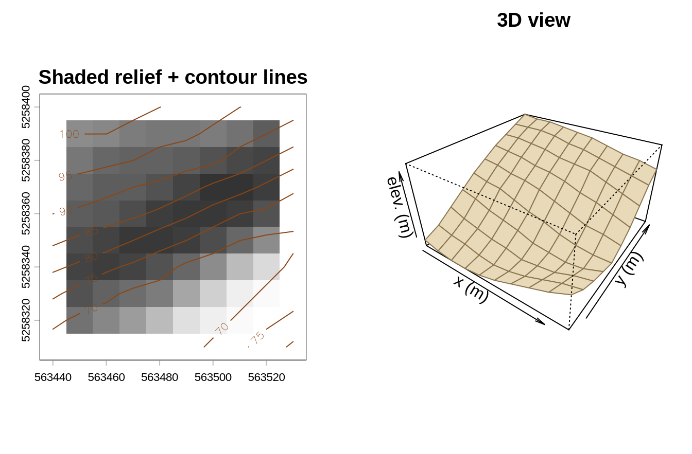
To build intuition before looking at the files one by one, here is the relief of the synthetic “watershed”:
Code
library(terra)dem <-rast("../exemplo_01/data/dem.asc")par(mfrow =c(1, 2), mar =c(2.5, 2.5, 2, 1))hs <-shade(terrain(dem, "slope", unit ="radians"),terrain(dem, "aspect", unit ="radians"))plot(hs, col =grey(seq(0.2, 1, length.out =40)), legend =FALSE,main ="Shaded relief + contour lines")contour(dem, add =TRUE, col ="#8b4513", labcex =0.7)persp(dem, theta =35, phi =32, expand =0.55, col ="#e8d9b8",border ="#8a7550", main ="3D view", xlab ="x (m)", ylab ="y (m)",zlab ="elev. (m)")
The synthetic terrain of the tutorial: shaded relief with contour lines (left) and 3D perspective view (right).
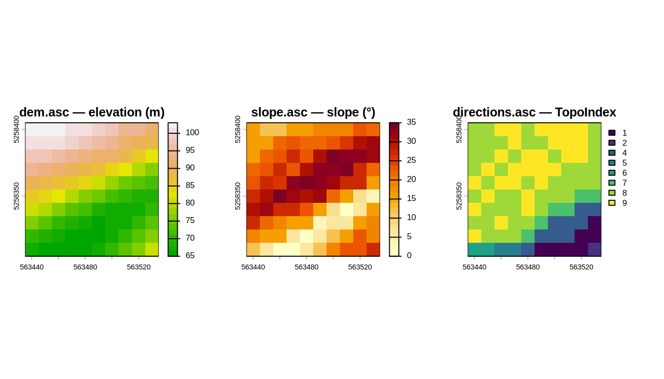
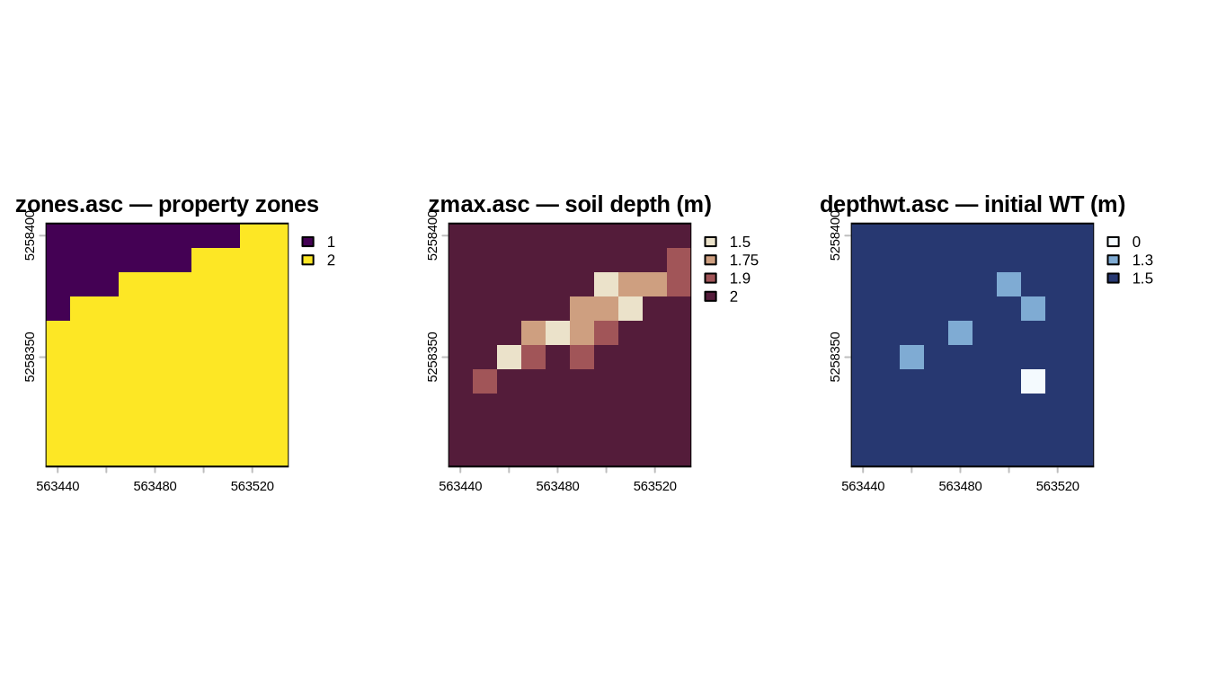
Each .asc file in the data\ folder answers one of the model’s questions. We will look at them in groups, always with the corresponding map next to the description.
rizero.asc — long-term antecedent infiltration (maintains the initial state);
ri1.asc, ri2.asc — rainfall intensity of each period, in m/s (read only when the corresponding cri value in tr_in.txt is negative — see the initialization files below).
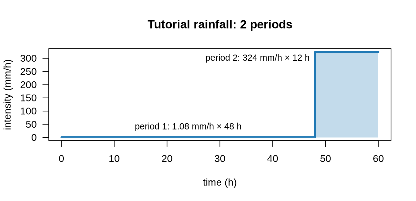
Rainfall enters TRIGRS as a stepped hyetograph: the total duration is divided into periods (nper in tr_in.txt), each with its own intensity — given as a uniform value or as an ri*.asc grid (spatially varying rainfall, e.g., interpolated from rain gauges or radar). The tutorial has two periods — 48 h of light antecedent rain and 12 h of a storm (deliberately exaggerated, to force instability on the tiny grid):
The tutorial hyetograph: the uniform intensities cri of tr_in.txt (3×10⁻⁷ and 9×10⁻⁵ m/s) converted to mm/h — being positive, they are used instead of the ri1 and ri2 grids. The final storm is unrealistic on purpose — it is a teaching dataset.
4.4 The initialization files
Each program reads a text file with parameters and paths, in the folder where it is run:
tpx_in.txt (TopoIndex): points to the DEM and to the flow-direction grid; sets the D8 scheme (ESRI = 1, TopoIndex = 2) and which auxiliary lists/grids to save.
tr_in.txt (TRIGRS): the heart of the run. Among other things, it defines:
the number of zones and the geotechnical/hydraulic parameters of each zone (cohesion in Pa, friction angle φ in degrees, unit weight in N/m³, diffusivity in m²/s, Ksat in m/s, θsat, θres, Gardner’s α);
rainfall periods (nper), switching times (capt), and intensities (cri or ri*.asc grids);
the simulation depth, the initial water-table condition, and the model options (saturated/unsaturated, finite/infinite depth);
output times and which grids to write.
A negative value of zmax, depth, rizero, or of an intensity cri tells TRIGRS to read the corresponding grid (zmax.asc, depthwt.asc, rizero.asc, ri*.asc) instead of using the value itself. In the tutorial, zmax = -3.001, depth = -2.4, and rizero = -1.0e-9, so these three grids are read; the intensities cri (3×10⁻⁷ and 9×10⁻⁵ m/s) are positive and are applied uniformly.
In the tutorial, the two zones of zones.asc receive these parameters (lines zone, 1 and zone, 2 of tr_in.txt):
Parameter (SI unit)
Zone 1
Zone 2
Role in the model
Cohesion c’ (Pa)
3,500
8,000
strength that does not depend on normal stress
Friction φ’ (degrees)
35
31
frictional strength
Unit weight γs (N/m³)
22,000
22,000
weight of the soil column
Diffusivity D₀ (m²/s)
6.0×10⁻⁶
8.0×10⁻⁴
speed of the pore-pressure response
Ksat (m/s)
1.0×10⁻⁷
1.0×10⁻⁴
infiltration capacity
θsat / θres
0.45 / 0.05
0.45 / 0.06
saturated/residual water contents
Gardner’s α (1/m)
−0.5
−8.0
K(ψ) curve of the unsaturated zone
Note the contrast: zone 1 has the higher friction angle but lower cohesion and is much less permeable (it responds slowly); zone 2 is more cohesive but has a lower friction angle and is much more permeable — the storm reaches it quickly. This interplay produces the instability pattern we will see in the next chapter.
4.5 Units — pitfall #1
TRIGRS works in SI units: meters, seconds, pascals. Rainfall enters in m/s: